
 Some Notes on Two-Element Horizontal Phased Arrays
In Part 1, we noted that there are two ways of looking at the idea of a phased array. One perspective views the phased array as a combination of elements, all of which are fed. The other perspective is more general: it examines the relative current magnitude and phase angle of element combinations, regardless of which one or more of them may be fed. From this latter perspective, a 2-element parasitic array is phased in the sense that the unfed element will display a relative current magnitude and phase angle.
The parasitic array, of course, has a more common name: the Yagi-Uda beam. The Yagi (for short) may have as many parasitic elements as a designer can put to good use. Our interest will be in the smallest of such arrays: 2-element models. Fig. 2-1 shows the options that we have for creating 2-element Yagis. We may either use a director or forward parasitic elements with a driven element, or we may use a reflector or rear parasitic element with a driven element.

The names "director" and "reflector" are simply conventional tags by which we identify a given parasitic element. The names do not themselves indicate how a parasitic array operates. Indeed, among those new to antennas, we find numerous misconceptions concerning reflectors, including the idea that they function similarly to the mirrored surface behind the light source in a flashlight. Directors, by the same analogy, appear to function in the manner of optical lenses by focusing the beam of RF.
Let's approach 2-element Yagis from a different point-of-view. The close proximity of the 2 elements provides significant inter-element coupling such that the unfed element will show at its center a relative current magnitude and phase angle. By adjusting the element diameters, spacing, and lengths, we may alter the unfed element relative current magnitude and phase angle. However, this process is limited by the basic geometry of the array. It is composed of parallel linear elements. Hence, the three variables of length, diameter and spacing can only go so far in yielding on the unfed element a relative current magnitude and phase angle that corresponds with those identified in Part 1 as able to produce a desired radiation pattern.
In this episode, we shall look more closely at the basic properties of 2-element Yagis in both the reflector-driver and the driver-director configuration. Our efforts will be to understand what limitations that geometry alone, as a set of design variables, places on the performance of 2-element arrays, especially compared to independently feeding both elements. When we are done, we should be able to correlate typical Yagi patterns with the relative phasing conditions for the two elements. At the end, we shall look at some alternative 2-element geometries designed to improve those conditions.
We shall also limit our samples to the same increments of element spacing that we used in Part 1: from 0.05 wl to 0.2 wl in 0.025-wl increments. Where our interest will depart from the earlier study is in the recording of the relative current magnitude and phase angle on the parasitic element when the driver has a current magnitude of 1.0 and a phase angle of 0.0 degrees.
                           2-Element Reflector-Driver Performance
                Set for Maximum 180-Degree Front-to-Back Ratio and Resonance

Element       Reflector     Driver         Gain          Front-to-Back        Feedpoint Z
Spacing wl    Length wl     Length wl      dBi           Ratio dB             R +/- jX Ohms
0.05          0.2505        0.2387         6.24          11.36                 8.1 + j 0.1
0.075         0.2507        0.2356         6.36          11.40                15.4 - j 0.2
0.1           0.2511        0.2334         6.32          11.33                24.3 - j 0.1
0.125         0.2514        0.2310         6.25          11.18                33.8 + j 0.0
0.15          0.2513        0.2312         6.18          10.96                42.9 - j 0.1
0.175         0.2513        0.2310         6.06          10.69                52.1 + j 0.0
0.2           0.2511        0.2312         5.91          10.36                60.2 - j 0.0

Note:  All elements 0.5" (0.001207 wl) aluminum

Table 1.  2-element reflector-driver Yagi performance when set for maximum 180-degree
front-to-back ratio and driver resonance.
Table 1 provides the basic performance data for the models of a reflector-driver parasitic array meeting the conditions we have just specified. In addition to the usual performance data (free-space gain in dBi, 180-degree front-to-back ratio in dB, and the source impedance in Ohms), the table provides element lengths as a function of a wavelength at the test frequency. Unlike the models in Part 1, which used a relatively arbitrary but consistent dimensions for each model, the parasitic array must have different element lengths at each increment of spacing to achieve the maximum front-to-back ratio at a resonant driver impedance.
The dimensions themselves hold some interest. As you scan the table, note that the reflector length required to meet the twin modeling objectives reaches a peak length at a spacing of 0.125 wl and then decreases. In contrast, the required driver length decreases until the element spacing is 0.175 wl and then increases.

Fig. 2-2 graphs the gain and front-to-back ratio data as a convenient way to examine the trends. Within the limitations of the increments of element spacing used here, the gain and the front-to-back ratio reach their peak values with an element spacing of 0.075 wl. As we shall see, there are two good reasons why we rarely, if ever, design 2-element reflector-driver Yagis with this particular spacing. One of those reason is the low source impedance: just above 15 Ohms. The other reason is the narrowness of the operating bandwidth at this spacing, a facet of 2-element Yagi design that we shall examine more thoroughly in a moment.
The low level of the front-to-back ratio of the reflector-driver design has struck many antenna enthusiasts and has occasioned two responses. One is the design of 3-element and larger Yagis. The second is the design of arrays that feed both elements. The front-to-back ratio with an element spacing of 0.125 wl is about 11.18 dB. We can increase this level to about 11.50 dB largely by shortening the driver and thereby changing the mutual coupling between the elements. However, in the process, the gain begins to decrease, and the source impedance reaches a value of about 30 - j 52 Ohms. Hence, draining the reflector-driver design of the last modicum of front-to-back ratio tends to result in relatively impractical source impedance values.
          Actual vs. Ideal Rear Element Relative Current Magnitude and Phase Angle
                              2-Element Reflector-Driver Yagis

                            Actual                                     Ideal
Element              Relative       Relative      Relative      Relative      Gain
Spacing wl           I Mag.         I Phase       I Mag.        I Phase       dBi
0.05                 0.833          165.1         0.963         163.1         6.51
0.75                 0.774          158.1         0.953         154.1         6.51
0.1                  0.719          150.7         0.944         144.9         6.44
0.125                0.670          143.1         0.938         135.6         6.33
0.15                 0.636          136.5         0.938         126.1         6.18
0.175                0.603          129.3         0.936         116.6         6.00
0.2                  0.576          122.4         0.937         107.1         5.77

Note:  all phase angles adjusted for positive values.  For negative angle values
corresponding to those in Part 1, subtract 180 from the listed value.  All "ideal
models" set to a 180-degree front-to-back ratio greater than 60 dB.


Table 2.  Actual vs. ideal rear element relative current magnitude and phase
angle values for maximum 180-degree front-to-back ratios for 2-element reflector-
driver Yagis in Table 1.
               Bandwidth Characteristics for 2-Element Reflector-Driver Yagis
                         At 0.1, 0.125, and 0.15 WL Element Spacing

Element Spacing:  0.1 wl
Frequency     Gain          Front-to-Back         Feedpoint Z                 SWR Relative
MHz           dBi           Ratio dB              R +/- j X Ohms              to 24.3 Ohms
28.0          6.84           9.53                 16.3 - j 23.1               3.20
28.25         6.58          10.94                 20.2 - j 11.3               1.71
28.5          6.32          11.33                 24.3 - j  0.1               1.01
28.75         6.07          11.01                 28.4 + j 10.4               1.53
29.0          5.86          10.41                 20.5 + j 20.5               2.16

Element Spacing:  0.125 wl
Frequency     Gain          Front-to-Back         Feedpoint Z                 SWR Relative
MHz           dBi           Ratio dB              R +/- j X Ohms              to 33.8 Ohms
28.0          6.72           9.92                 24.7 - j 21.4               2.19
28.25         6.48          10.91                 29.3 - j 10.3               1.43
28.5          6.25          11.18                 33.8 + j  0.0               1.00
28.75         6.04          10.94                 38.1 + j  9.8               1.35
29.0          5.85          10.45                 42.3 + j 19.2               1.73

Element Spacing:  0.15 wl
Frequency     Gain          Front-to-Back         Feedpoint Z                 SWR Relative
MHz           dBi           Ratio dB              R +/- j X Ohms              to 33.8 Ohms
28.0          6.61           9.89                 33.3 - j 20.0               1.78
28.25         6.39          10.71                 38.1 - j  9.7               1.31
28.5          6.18          10.96                 42.9 - j  0.1               1.00
28.75         5.98          10.80                 47.4 + j  9.0               1.25
29.0          5.80          10.41                 51.7 + j 17.7               1.52


Table 3.  Bandwidth characteristics for 2-element reflector-driver Yagis at 0.1,
0.125, and 0.15 wl element spacing.
Table 2 reveals the reason for the low levels of front-to-back ratio associated with reflector-driver Yagi designs. The table lists the modeled rear-element relative current magnitude and phase angle values, along with the values needed for the same set of elements to achieve more than 60 dB front-to-back ratio. (The ideal front-to-back ratio models show the same deep 180-degree null as those in Part 1, along with the rearward side lobes that result in worst-cast front-to-back ratios between 17 and 22 dB.) The gain of the models using two sources appear in the right-most column. The ideal phase angles have been converted from the negative angles typical of models in Part 1 to values that correspond to those yielded by models of Yagis. To convert either value to more suited to phasing networks, simply subtract 180 degrees from the listed value.
In concert with the curves that we saw in Fig. 2-2, the relative current magnitude and the phase angle of the optimized Yagi both depart more radically from the ideal numbers with the widening of the spacing between elements. Coincidence is closest at the narrowest spacings. However, the narrower the spacing between elements, the more exact the coincidence must be to yield the ideal maximum front-to-back value of more than 60 dB. Hence, the closeness of the values at a spacing of 0.05 wl is still not close enough to yield the highest front-to-back ratio. As well, the ideal model shows its highest gain at the narrowest spacing, although the Yagi does reach maximum gain until the spacing is 0.075 wl. Interestingly, the ideal models have a higher gain potential only until the spacing reaches 0.15 wl, after which the Yagi shows slightly higher gain.
                            2-Element Driver-Director Performance
                Set for Maximum 180-Degree Front-to-Back Ratio and Resonance

Element       Driver        Director       Gain          Front-to-Back        Feedpoint Z
Spacing wl    Length wl     Length wl      dBi           Ratio dB             R +/- jX Ohms
0.05          0.2498        0.2378         6.48          26.03                11.0 - j 0.0
0.075         0.2486        0.2335         6.52          23.60                21.1 + j 0.2
0.1           0.2465        0.2298         6.44          14.85                29.7 + j 0.2
0.125         0.2443        0.2263         6.22          10.66                36.6 + j 0.1
0.15          0.2423        0.2234         5.98           7.94                41.2 + j 0.2
0.175         0.2407        0.2202         5.62           5.96                45.9 + j 0.1
0.2           0.2395        0.2170         5.23           4.45                50.0 + j 0.2

Note:  All elements 0.5" (0.001207 wl) aluminum

Table 4.  2-element driver-director Yagi performance when set for maximum 180-
degree front-to-back ratio and driver resonance.
If we shift to driver-director models of parasitic arrays, we do not get the same picture of results. Table 4 lists the element lengths and the basic performance figures for the driver-director configuration. Unlike the reflector-driver dimensions, the driver-director element lengths continuously decrease with increased spacing between elements.

The table also confirms the general proposition that a driver-director array develops a significant gain and front-to-back superiority over the reflector-driver array when the spacing is fairly narrow--under 0.1 wl. Fig. 2-3 tracks the gain and front-to-back ratio values. Above 0.1 wl element spacing, the front-to-back ratio drops rapidly to the reflector model values and below. The gain values start their drop above 0.75-wl spacing. Since the 21-Ohms impedance of the 0.075-wl model is manageable with a matching network, this element spacing region is among the most popular for driver-director arrays.
The flatted curve between 0.05-wl and 0.075-wl element spacing hides a surprise for those not familiar with Jerry Hall's study. The slope of the curve beyond the 0.075-wl mark suggests that in the lowest region of spacing, there is a peak in the front-to-back value. In fact, at a spacing of 0.0625 wl, the front-to-back ratio can reach nearly 47 dB with a free-space gain of 6.52 dBi and a source impedance of about 16.5 + j 7.9 Ohms. Such an array also comes closest to meeting the ideal conditions for maximum front-to-back ratio, with a relative magnitude of 0.964 and a phase angle (adjusted) of 158.6 degrees (or -21.4 degrees). For single-frequency use, such an array might well fill a need.
          Actual vs. Ideal Rear Element Relative Current Magnitude and Phase Angle
                               2-Element Driver-Director Yagis

                            Actual                                     Ideal
Element              Relative       Relative      Relative      Relative      Gain
Spacing wl           I Mag.         I Phase       I Mag.        I Phase       dBi
0.05                 0.934          162.8         0.961         163.1         6.51
0.75                 1.006          149.5         0.951         154.1         6.51
0.1                  1.140          149.7         0.948         144.9         6.43
0.125                1.333          146.1         0.943         135.5         6.31
0.15                 1.555          145.6         0.939         126.1         6.16
0.175                1.845          145.8         0.926         116.7         5.96
0.2                  2.188          147.3         0.910         107.3         5.72

Note:  all phase angles adjusted for positive values.  For negative angle values
corresponding to those in Part 1, subtract 180 from the listed value.  In
addition, actual angles are taken from the director and appear as negative angles
relative to the driver to the rear.  The relative current magnitude values have
been adjusted to reflect the values on the rear element if the forward element
is set at 1.0.  All "ideal models" set to a 180-degree front-to-back ratio
greater than 60 dB.


Table 5.  Actual vs. ideal rear element relative current magnitude and phase
angle values for maximum 180-degree front-to-back ratios for 2-element driver-
director Yagis in Table 3.
                Bandwidth Characteristics for 2-Element Driver-Director Yagis
                         At 0.075, 0.1, and 0.125 WL Element Spacing

Element Spacing:  0.075 wl
Frequency     Gain          Front-to-Back         Feedpoint Z                 SWR Relative
MHz           dBi           Ratio dB              R +/- j X Ohms              to 21.1 Ohms
28.0          5.59          12.31                 33.0 - j 21.6               2.47
28.25         6.03          16.75                 27.0 - j 11.6               1.72
28.5          6.52          23.60                 21.1 + j  0.2               1.01
28.75         7.00          15.47                 15.7 + j 13.9               2.22
29.0          7.30           8.87                 11.6 + j 29.2               5.66

Element Spacing:  0.1 wl
Frequency     Gain          Front-to-Back         Feedpoint Z                 SWR Relative
MHz           dBi           Ratio dB              R +/- j X Ohms              to 29.7 Ohms
28.0          5.64          11.39                 39.2 - j 19.5               1.87
28.25         6.03          13.54                 34.7 - j 10.3               1.43
28.5          6.44          14.85                 29.7 + j  0.2               1.01
28.75         6.84          12.96                 24.6 + j 12.4               1.63
29.0          7.15           9.28                 20.1 + j 26.4               2.98

Element Spacing:  0.125 wl
Frequency     Gain          Front-to-Back         Feedpoint Z                 SWR Relative
MHz           dBi           Ratio dB              R +/- j X Ohms              to 36.6 Ohms
28.0          5.55           9.35                 43.2 - j 18.7               1.64
28.25         5.87          10.24                 40.2 - j  9.8               1.31
28.5          6.22          10.66                 36.6 - j  0.1               1.00
28.75         6.56          10.05                 32.7 + j 11.1               1.40
29.0          6.84           8.36                 28.8 + j 23.7               2.11


Table 6.  Bandwidth characteristics for 2-element driver-director Yagis at 0.075,
0.1, and 0.125 wl element spacing.
Table 5 provides data comparing the modeled relative current magnitude and phase angle for the unfed element. The data has been adjusted to coincide in form with other data that we have examined. The negative phase angles of the director have been made positive, as if the forward element had a value of 0.0 degrees. As well, the current magnitude has been adjusted as if the director had a value of 1.0. This set of adjustments allows the ideal data to correspond with all other dual-source models we have so far examined, where all forward elements are set to a magnitude of 1.0 and a phase angle of 0.0 degrees, and the rear element values are presented for comparison. In concert with the curves of Fig. 2-3, Table 5 makes evident the rapid departure from ideal phasing conditions for maximum front-to-back ratio above 0.075-wl element spacing. Equally evident, in comparison with the data for the reflector-driver Yagi, is the relative uselessness of the driver-director array as a directional beam able about 0.1-wl element spacing.

Despite the radical differences in gain and front-to-back behavior between reflector-driver and driver-director Yagis, the resonant impedances of the two arrays do not differ greatly for any given element spacing. Fig. 2-4 tracks the source resistance of the two array designs as optimized for each element spacing increments. An interesting property of reflector-driver designs is that the impedance curve is nearly linear, in contrast to the curve for the driver-director array.

In our exploration of the two types of parasitic arrays, we overlooked Table 3 and Table 6. These tables present modeled performance figures for each array at 3 increments of element spacing from 28.0 to 29.0 MHz. For each array, the most common element spacings are listed: 0.1 through 0.15 wl for the reflector-driver array and 0.75 through 0.125 wl for the driver-director Yagi. As expected, operating bandwidth increases with increased element spacing. The reflector-driver Yagi, shown in Fig. 2-5, can be adjusted to cover the entire 1-MHz bandwidth by selecting a design frequency of about 28.35 rather than the 28.5-MHz figure used in this study. At a slightly wider element spacing of 0.15 wl, the 2-element reflector-driver design can be designed to cover all of the 10-meter band. At each level of element spacing, the gain and the front-to-back values tend to show the same sort of curve broadening with each increase in spacing, although the peak values decrease along the way.

The driver-director Yagi SWR curves, shown in Fig. 2-6, are naturally steeper, given the narrower element spacings involved. The most notable feature of the SWR graph is it reversal from the one for the reflector-driver array: here, more rapid increases occur above the design frequency rather than below it. Likewise, gain increases with rising frequency (rather than with decreasing frequency in the case of the reflector-driver array). The source impedance of the driver-director array shows an increasing reactance with frequency in accord with the relative shortening of the element. However, the resistive component of the impedance decreases with rising frequency (in contrast to the resistance curve of the reflector-driver Yagi). At the spacing increments generally used in driver-director designs, narrow bandwidth is a condition of maximizing performance.
Understanding basic 2-element Yagi-Uda performance is a necessary condition of understanding the urge to design phased arrays in which both elements are fed. In principle, the dual source phased array is capable of higher gain and better front-to-back performance than all but the most closely spaced parasitic arrays. The reason is simple: the wider the spacing of a parasitic array, the further the elements get from relatively ideal conditions of element current magnitude and phase angle.

The Moxon rectangle owes its operating characteristics to not one, but two forms of inter-element coupling. Between the parallel portions of the elements, we encounter the same sort of mutual coupling that is almost the sole source of coupling within a standard Yagi design. However, by bending the elements toward each other, we obtain an added form of coupling, often called capacitive coupling between the element ends. The result is a broader beamwidth and an increase in the front-to-back ratio. By judicious control of the element diameter, the gap between element tails, and the other dimensions of the array, we may obtain a broad-band reflector-driver array.

Fig. 2-8 shows the free-space gain and front-to-back curve for a typical Moxon rectangle designed for 28.35 MHz using 0.5" aluminum elements. The design frequency is necessary, since reflector-driver arrays decrease their front-to-back ratio and increase their SWR more slowly above the design frequency than below it. The resulting array covers the first MHz of 10 meters. The gain decreases nearly linearly across the passband, while the front-to-back ratio peaks just below the 28.4-MHz mark on the graph. Fig. 2-9 shows the 50-Ohm SWR curve for the design.
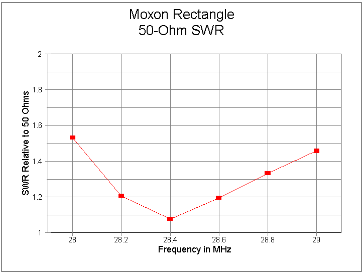
Since Moxon rectangle designs using a variety of element materials and design frequencies are now common in antenna literature, we may turn our attention to Table 7. This table summarizes the performance data shown in the graph. In addition, it provides values for the rear element relative current magnitude and phase angle. At the design frequency, the parallel portions of the elements are about 0.133 wl apart. At that spacing, an ideal phase angle would be about 132.5 degrees (or -47.5 degrees). The rear element relative current magnitude would be close to 0.94. Compare these values to the ones in the table for 28.2 (0.967 and 134.1 degrees) and 28.4 MHz (0.943 and 128.0 degrees). Little wonder that the Moxon rectangle achieves a maximum front-to-back ratio of well over 30 dB at its design frequency.
                   Bandwidth Characteristics for 2-Element Moxon Rectangle

Frequency     Gain   Front-Back     Feedpoint Z          50-Ohm        Refl.          Refl.
MHz           dBi    Ratio dB       R +/- j X Ohms       SWR           I Mag.         I Phase
28.0          6.36   17.79          39.2 - j 15.7        1.53          0.980          140.1
28.2          6.16   25.95          46.3 - j  8.3        1.21          0.967          134.1
28.4          5.95   34.12          53.2 - j  2.2        1.08          0.943          128.0
28.6          5.75   22.21          59.3 + j  2.9        1.20          0.911          122.5
28.8          5.57   17.81          64.6 + j  7.3        1.33          0.874          117.6
29.0          5.40   15.20          69.2 + j 11.4        1.46          0.835          113.2

Note:  Aluminum element diameter:  0.5"  (0.001207 wl)

Table 7.  Bandwidth characteristics for 2-element Moxon rectangle, with modeled
rear element relative current magnitudes and phase angles.
The cost for this improved front-to-back figure is a decrease in gain, partly resulting from the increased beamwidth relative to a standard Yagi design. Since the bent portions of the elements still have significant current levels near the array corners, their contribution to gain becomes a contribution to beamwidth. Hence, the Moxon rectangle has an average free-space gain of about 6.0 dBi, somewhat below the levels of the optimized Yagis and of the idealized phased arrays that we examined in Part 1.

The Moxon rectangle is not the only attempt to alter geometry to improve performance over parallel-element Yagis. Fig. 2-10 shows some of the other arrangements tried with greater or lesser success. The VK2ABQ square was a forerunner of the Moxon rectangle. The diamond lends itself to inexpensive construction with a single non-conductive support for wire element ends. The hex and folded-X have been popular from time to time as near-ultimate compact but full size designs. An interesting study, but beyond the scope of these notes, would be to investigate the relative current magnitude and phase on the unfed element in each design, noting that the most common implementation of the folded X-beam is as a driver-director array. The others are all reflector-driver arrays.
The key to 2-element Yagi design shortcomings is also the key to 2-element horizontal phased array success. Can we find a practical way to implement a 2-element phased array with both elements fed to arrive at desired gain, front-to-back ratio, and bandwidth values? In the next episode, we shall begin our exploration by reviewing the ZL-Special and its variants, all of which make use of what seems in principle to be the simplest phasing mechanism possible: a single phasing line that connects the two elements. More complex systems, such as the HB9CV and the N7CL systems do exist, but basic principles of phasing are often best explored by keeping the number of design variables to a minimum. The more complex systems will have their turn in Part 4.
Updated 01-12-2002. © L. B. Cebik, W4RNL. This item originally appeared in The National Contest Journal (Jan/Feb, 2002). Data may be used for personal purposes, but may not be reproduced for publication in print or any other medium without permission of the author.