 What Can We Expect from a 2-Element Beam?
Let's look at some of the strategies for improvement and divide the work into 2 parts: strategies that can improve front-to-back ratio and strategies that may improve both the gain and the front-to-back ratio. Additionally, we shall look at only some samples of strategies, because the total number of ways to go about the process is limited only by the antenna designer's imagination. However, we shall be able to note some very interesting general trends.
The 2-Element Phased Array: I have done an extensive study of the ZL Special, in "Understanding and Modeling Small Beams: Part 5: The ZL Special," Communications Quarterly, (Winter, 1997), 72-90. The ZL Special became popular in the 50s after a series of articles by ZL3MH/ZL2QQ, George Prichard, with some quick test work by G2BCX. Claims of 7 dBd gain and 40 dB front-to-back ratios were common, mostly because the antenna outperformed many of the ill-designed 3-element Yagis of the period. It remained almost a constant claim that the antenna was a phased array 1/8 wavelength separated and using a twisted 45-degree phase line to give 135-degree phasing. It was Roy Lewallen who pointed out in the 1980s that is was not the impedance at the rear element that was critical, but the current, and this changed the analysis ball game, although it appears few have taken up the challenge.

The ZL-Special is only one of several types of the 2-element horizontal phased arrays, and Fig. 1 does not show all of the possibilities. While the ZL-Special, with a single phase-line, is popular in the U.S and in the British Commonwealth, the HB9CV, with 2 phase lines fed at the center point between elements is popular in the rest of Europe. Due to the impedances of the lines and the elements, it usually requires a gamma match at each element. A much simpler double phase-line arrangement appears under the title "modified." The two lines have unequal lengths, with the feedpoint at the junction of the two lines. It achieves the same goal as the other two designs, but allows the use of common transmission lines, such as coaxial cable, as the phase line. The variety of phasing techniques led me to do a multi-part study for The National Contest Journal a few years ago, and the episodes are at this website. See "Some Notes on Two-Element Horizontal Phased Arrays." Note that in Fig. 1, we do not refer to the elements as a driver and reflector, since we are driving both elements. In fact, both elements receive energy via direct feed and by coupled energy from the other element. Generally, we call the element in the direction of the forward lobe element 1 and the rearward wire element 2.
Since current goes through a 360-degree cycle, not a 180-degree cycle like impedance along a transmission line, the proper analysis of a one-line ZL-Special must treat it as a -45-degree phased array. The minus sign is the product of the phase line twist. Once we make this shift in perspective, we can analyze the relationships of the current magnitudes and phases along the line such that they yield correct values for the spacing used and wind up with identical voltage magnitudes and phases at the junction with the feedline. For a given situation, line length, characteristic impedance, and velocity factor combine so that few values will satisfy the requirements, and fewer still if we stick to available commercial lines.
The spacing need not be precisely 1/8 wavelength, since every spacing between a very small one and something just under 1/4 wavelength has a current magnitude and phase requirement for the rear element that will yield maximum front-to-back ratio. In fact, for 1/8 wavelength spacing, the current phasing must be about -43-44 degrees, at 0.1 wavelength spacing, the current phasing must be about -34 degrees, and at 0.15 wavelength spacing, the current phase must be about -53 degrees. A similar analysis applies to other types of phased arrays. Indeed, the goal of the phase lines, if we have more than one of them, is to establish the relative current magnitude and phase relationship required for a desired pattern based on the length of the two elements and on the spacing between them. The element diameter will have a small but noticeable effect on the process, since it also affects the mutual coupling between elements.
In general, a pair of phased horizontal elements is not capable of a maximum forward gain in excess of about 7.1 dBi in free space. That gain level is approximately the peak gain of the 2-element parasitic Yagi when set for maximum gain. Like the maximum-gain Yagi, the phased array--when set for maximum gain--has a very poor front-to-back ratio, usually well below 10 dB. The phased element pair, however, can achieve a much higher front-to-back ratio than the parasitic driver-reflector Yagi. Because we can control the current magnitude and phase-angle relationship between the two elements, we can reach front-to-back levels as high as 50 dB at a design frequency. The high front-to-back ratio has several limitations. First, it occurs at a specific frequency and decreases immediately as we move above or below that frequency. Second, the gain the accompanies the maximum front-to-back ratio is slightly less than we can get from driver-reflector Yagis with element spacing values between 0.12 and 0.16 wavelength.
For these reasons, most serious phased-array designer aim for a middle ground between maximum gain and maximum front-to-back ratio. There is a middle ground that shows a small gain improvement but a considerable (8 to 10 dB) front-to-back ratio improvement over the driver-reflector Yagi. The benefit of designing in this region is that one can usually spread the benefits over a sizable operating bandwidth.
As a sample phased array, let's look at a design that I published several years ago using different element structures than the 3/8" aluminum elements used throughout this series of notes. One interesting feature of this design is that we can use the beam as a reflector-driver Yagi or as a phased array with a variety of phase-line arrangements. Fig. 2 shows the basic outline of the array.

Element 1 or the driver is 16.13' long, while the reflector or element 2 is 17.41' long. The spacing between elements is 4.8' or 0.139 wavelength. This spacing is at the edge of the Yagi broadband spacing range and allows a direct 50-Ohm feedpoint when we use the antenna in this mode.
When we wish to convert the antenna into a phased array, we have at least 2 choices, We can use a single 35-Ohm cable (RG-83) in ZL-Special style. The line length will be 4.83' for a cable with 0.66-velocity factor (VF). The resulting feedpoint impedance at the junction of the phase line with the forward element is close to 25 Ohms. So we need a roughly quarter wavelength matching section (5.69') of 35-37-Ohm, 0.66-VF line. We can make up such a line with parallel sections of RG-59 cable. If we cannot obtain 35-Ohm cable for the phase line, we can use 50-Ohm RG-8X with a velocity factor of 0.78. However, we need two sections. A 6" section goes from the feedpoint junction to the forward element, while a 64" (5.33') section goes from the junction to the rear element. The impedance at the junction will not be identical to what we obtain from the 35-Ohm phase line, but a 34" (3') matching section of paralleled RG-59 will yield a 50-Ohm match.

The performance difference between the Yagi and phased modes of operation shows up in the overlaid patterns in Fig. 3 at the design frequency of 28.5 MHz for this antenna. The phased version has about 1/3-dB higher gain, but the main benefit occurs in the rearward direction. The phased version has double the front-to-back ratio of the Yagi version. For a broader view of the antenna's performance, Table 1 presents modeled free-space values at 28 and 29 MHz as well as at the design frequency.
Table 1.  Performance of a two element array as a Yagi and as a phased-array

Antenna                          Frequency (MHz)
               28                  28.5                29
Yagi
Gain (dBi)     6.61                6.14                5.74
F-B (dB)       10.06               11.01               10.21
Feed Z         30.6 - j17.1        40.5 + j4.4         49.4 + j23.7
50-Ohm SWR     1.91                1.26                1.61

Phased Array
Gain (dBi)     6.00                6.50                6.99
F-B (dB)       21.02               22.91               12.51
Feed Z         75.9 - j12.5        51.4 - j9.3         32.7 + j5.5
50-Ohm SWR     1.59                1.20                1.56
Both versions of the antenna offer very good SWR curves for a 50-Ohm cable across the entire first MHz of 10 meters. Fig. 4 provides the modeled SWR values in 0.1-MHz increments. Note that the Yagi version requires no matching section, but the phased array version requires both a phase line and a matching section. The fact that the phased array version shows a descending feedpoint resistance as the frequency increases results from the impedance transformation within the matching section.

The gain curves for the two antenna show opposite trends, as is evident in Fig. 5. The Yagi shows the typical driver-reflector trend of decreasing gain with increasing frequency. In contrast, the phased array shows increasing gain with frequency, a trend that is more typical of parasitic Yagis with one or more directors.

Fig. 6 shows the two front-to-back curves for the Yagi and the phased array. The Yagi curve is very flat across the entire passband for the antenna. In contrast, the phased array shows a definite peak. Because the phased array is an adapted use of a Yagi design, the peak does not occur at the design frequency, but about 200 kHz lower. Still, the front-to-back ratio remains higher than the value for the Yagi throughout the operating passband. However, we note in passing that as the gain approaches the 7-dBi mark, the front-to-back ratio is in serious decline.

The sample phased array has provided us with a good sample of typical performance and a good comparison with a comparable driver-reflector Yagi. Since there are so many ways to handle the phasing and matching requirements of phased arrays, other sampled arrays will yield other results. However, all will fall within the limits of what is possible for phasing with 2 elements.
The Moxon Rectangle: What the phased array does with phasing lines, the Moxon rectangle does with geometry, that is, establish the correct rear element current magnitude and phasing for maximum front-to-back ratio. Derived from the VK2ABQ square, which is actually a rather poor performer, but with a germinal insight, the G6XN modification arose from practical considerations rather than a through understanding of what was going on. In fact, Moxon himself used the antenna with remotely tuned elements in order to flip the direction, and did not provide any solid basic information on its design. That led me to a considerable study of the antenna. See "Modeling and Understanding Small Beams: Part 2: VK2ABQ Squares and Moxon Rectangles," Communications Quarterly, (Spring, 1995), 55-70. Since that time, the Moxon rectangle has evolved steadily as a 50-Ohm 2-element beam. There are numerous articles at the web site on various aspects of Moxon rectangle design, assembly, and application. See the general listing called "Moxon Rectangles and Online Calculator" for a list of available articles.
The Moxon rectangle bends the forward and rear elements of a Yagi toward each other, with a small but critical space between the ends. The precise dimensions are a matter of design goal choice. Broader bandwidth of the front-to-back ratio occurs with squarer versions, but at a higher feedpoint impedance (80 ohms or so). One can also build versions that are narrow from front to back, and hence a bit wider from side to side, and achieve a 50-Ohm feedpoint impedance, although the front-to-back ratio goes down toward the edges of a frequency sweep. Models can be built with anything from wire to aluminum tubing. I have also developed a set of algorithms for designing Moxon rectangles from uniform-diameter elements from wire-size to fat tubing that covers the HF, VHF, and UHF ranges.
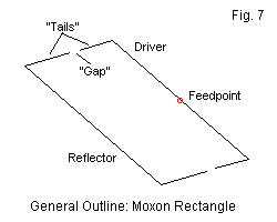
Fig. 7 shows the outline of a Moxon rectangle for a direct 50-Ohm coaxial-cable connection. Because we have bent the elements, the side-to-side dimension is only about 70% of the length of comparable Yagi elements. For an element diameter of 3/8", the dimension for 28.5 MHz model is 150.3" or 12.54'. The spacing between the driver and the reflector is 55.5" or 4.63'. The driver tails are 21.0". Hence, the total driver length is 192.3" or 16.03'. The reflector tails are 28.6" long, for a total reflector length of 207.5" or 17.29'. Note that the overall element lengths are not far distant from lengths that we meet with driver-reflector Yagis with linear elements. However, the operation of the Moxon depends on the element bends and the second form of coupling formed by the gap between the tails. The gap distance depends on the element diameter. Our 3/8" elements require a 5.9" gap at 28.5 MHz.
In one sense, the Moxon has slightly less forward gain than a 2-element Yagi or a phased, about 0.3-0.5-dB down on average. However, that gain applies over a much wider beamwidth. A typical 2-element Yagi has a beamwidth between half-power (-3dB) points of about 70 degrees. Moxon half-power points are typically 80 degrees or more apart, and the pattern circle extends beyond the 90-degree side direction. Hence, the proper application of a Moxon is where one wishes a broad forward hearing area and silence from the rear. It is ideal in the US for stations on the coast wanting to work the US without QRM from DX--or to work the DX across the water with silence from the US. Fig. 8 shows the patterns from the sample Moxon rectangle across the first MHz of 10 meters.

The figure presents 4 patterns rather than the usual 3 for an interesting reason. Both the front-to-back ratio and the SWR grow worse than ideal at a slower rate above the actual design frequency than below it. Hence, to obtain roughly equal front-to-back and SWR values at both the upper and lower operating frequency limits, the best design frequency is between 0.35 and 0.4 of the passband width above the lower end. For the sample model, I chose 28.35 MHz, the frequency that yields the best SWR and the best front-to-back ratio. As Table 2 shows, I came close to but did not hit the precise frequency that would yield equal performance values at both 28 and 29 MHz.
Table 2.  Modeled free-space performance of a Moxon rectangle

Frequency      28                  28.5                29

Gain (dBi)     6.43                5.87                5.39
F-B (dB)       16.96               26.21               14.88
Feed Z         38.2 - j16.3        56.3 + j1.1         69.8 + j12.6
50-Ohm SWR     1.58                1.13                1.48

Fig. 9 translates the data into graphical form for the forward gain and the front-to-back ratio. The gain curve shows the typical trend of a parasitic driver-reflector array. The front-to-back curve does not show the peak value because that value occurs between sampling points. However, the curve amply illustrates the more rapid decline in the front-to-back ratio below the design frequency than above it.

The 50-Ohm SWR curve in Fig. 10 mirrors the front-to-back curve. The Moxon rectangle has a broad SWR curve that makes the beam fairly easy to replicate successfully in a home workshop. Of course, the SWR passband will vary with the element diameter used, with wire showing a steeper curve and fatter elements (such a 1") showing a flatter curve across the first MHz of 10 meters.
The dual coupling between element ends and between the parallel portions of the elements does with antenna geometry much of what a phasing line does in a phased array. That is, it sets (on the design frequency) nearly ideal current magnitude and phase angle relationships that yield a very high front-to-back ratio. Because the geometry that yields the correct current magnitude and phase on the rear element to maximize front-to-back and front-to-rear ratio is frequency specific, the ratio falls off more rapidly than with the phased array sampled earlier--which was purposely not design for absolutely maximum front-to-back ratio. However, the Moxon rectangle remains superior to a standard 2-element Yagi driver-reflector array across the entire frequency sweep. It does all this from an antenna about 3/4ths the size of a standard Yagi.
Other designs have also been used to increase the front-to-back performance of the 2-element Yagi, but these two designs reveal what is at stake in making them work.
Table 3.  The effect of element diameter on 2-element driver-reflector Yagi performance

Element        Gain      F-B ratio      Feed Z
inches         dBi       dB             R +/- jX Ohms

Full size; 0.16 wl spacing
0.375          6.12      10.86          46.67 - j0.35
0.75           6.15      10.89          46.01 - j0.31
1.50           6.15      10.92          45.34 - j0.64
3.00           6.15      10.95          44.62 - j0.39

Fill size; 0.12 wl
0.375          6.25      11.19          32.47 + j0.23
0.75           6.31      11.23          31.33 - j0.98
1.50           6.31      11.27          31.08 - j0.52
3.00           6.30      11.31          30.74 - j0.99
Clearly, elements with diameters larger than 3/4" add virtually nothing more to the gain of the antenna. In each case, the beams in question used re-sized element lengths to achieve the best combination of gain and front-to-back ratio. As the element diameter grows, the required length decreases. As we learned early on with respect to dipole, shortening the dipole reduces its gain. At a certain point, the gain increase resulting from increasing element diameter crosses the gain decrease resulting from reduced length. Hence, the tactic becomes self-defeating beyond a certain point.
An alternative is to give up operating bandwidth and front-to-back ratio in favor of higher gain over a narrower passband. In our exploration of full-size reflector-driven element Yagis, we saw that the closer the elements, the higher the gain of the antenna. We need only review the antennas when the elements are spaced 0.08 (2.8') and 0.12 (4.1') wavelengths: see Table 4.
Table 4.  Relative performance of driver-reflector Yagis with closely spaced
and moderately spaced elements

Frequency      28        28.5      29        29.5      30  MHz

Maximum front-to-back-ratio designs

0.08 wl spacing
Gain (dBi)     6.37      6.92      6.32      5.77      5.37
F-B (dB)       1.82      8.65      11.38     10.12     8.57
SWR            31.2      5.88      1.04      2.91      5.52

0.12 wl spacing
Gain (dBi)     6.98      6.74      6.25      5.82      5.48
F-B (dB)       5.46      9.79      11.19     10.37     9.18
SWR            7.12      2.33      1.01      1.81      2.76

Maximum gain designs

Frequency      28        28.5      29        29.5      30  MHz
0.08 wl spacing
Gain (dBi)     7.15 R    6.01 R    7.02      6.59      6.02
F-B (dB)       10.29     0.72      6.29      10.61     10.54
SWR            40.6      16.4      1.01      6.87      14.2

0.12 wl spacing
Gain (dBi)     6.94 R    6.13      6.99      6.70      6.24
F-B (dB)       4.74      1.05      6.12      9.80      10.87
SWR            14.7      5.20      1.01      3.03      5.43
If a higher gain is desired and the conditions of obtaining it are acceptable, then a 2-element driver-director Yagi may serve the purposes at hand. Due to its narrow operating passband, the driver-director 2-element Yagi has restricted use. It is most apt for covering one of the narrow amateur bands, such as 30, 17, or 12 meters. In addition, amateurs who wish specialized antennas to cover only the CW-digital part or the SSB part of a wider amateur band may sometimes find the 2-element driver-director Yagi suitable.
The Driver-Director 2-Element Yagi A director plus driven element is capable of higher gain at close spacing values than a reflector plus driven element. The general outline of this Yagi type appears in Fig. 11.

If we use 3/8" aluminum elements (to be consistent with all of the other beam designs in these notes), we can optimize a series of 2-element driver-director Yagis at 29 MHz using different values of element spacing from 0.06 wavelength (2.03') up to 0.14 wavelength (4.75') on 0.02 wavelength intervals. The results of our first step appear in Table 5. Each version of this type of Yagi has been optimized for maximum front-to-back ratio at the design frequency.
Table 5.  Dimensions and 29-MHz performance of 2-element driver-director Yagis in free space

El. Spacing (WL/feet)          0.06 / 2.03     0.08 / 2.71     0.10 / 3.39     0.12 / 4.07     0.14 / 4.75
Driver Length (WL/feet)        0.474 / 16.07   0.467 / 15.85   0.462 / 15.66   0.457 / 15.50   0.452 / 15.34
Director Length (WL/feet)      0.499 / 16.92   0.497 / 16.85   0.494 / 16.74   0.490 / 16.62   0.487 / 16.52
Gain dBi                       6.51            6.50            6.42            6.32            6.12
Front-to-Back Ratio dB         45.18           20.95           14.83           11.33           8.91
Feed Z (R +/- jX)              14.82 - j0.11   22.98 + j0.06   29.69 + j0.16   34.53 - j0.05   38.94 + j0.20
As we increase the spacing between the elements, the lengths of both the driver and the director decrease. In addition, the gain also decreases as we increase the spacing between elements. The gain values at 0.12 wavelength and at 0.14 wavelength closely resemble the values that we might obtain from a driver-reflector Yagi.
Perhaps the most notable feature of the driver-director Yagi is the front-to-back ratio. If we use a close spacing value that is less than 0.10 wavelength, we can exceed the front-to-back ratio that we can obtain from the most common designs of the driver-reflector version of the Yagi. However, we pay a price: the resonant feedpoint impedance decreases to levels that we may find more difficult to match without also incurring losses.

Fig. 12 overlays sample patterns from the 0.06-, 0.10-, and 0.14 wavelength versions of the antenna. The overlay shows the development of the rearward radiation pattern, and you may easily interpolate the patterns for the missing plots (that would have made the overall graphic difficult to read). Note especially the rearward pattern for the smallest element spacing. Although the 180-degree front-to-back ratio is about 45 dB, the worst-case value at the center of each rearward lobe would be closer to 20 dB. The radiation in these directions does not change in strength as we increase the spacing. As a consequence, the best compromise design spacing might be in the vicinity of 0.08 wavelength, a value that yields a 21-dB 180-degree front-to-back ratio. This value would also approximate the worst-case value and the average values of front-to-back ratio over the entirety of the rearward quadrants. At the same time, the feedpoint impedance is about 23 Ohms, a value that is well within the ability of either a gamma or a beta match to provide a relatively low-loss matching system for a 50-Ohm feedline. Finally, the 0.08 wavelength spacing also provides a bit of added forward gain relative to common driver-reflector Yagi designs.
So far, we have examined the driver-director Yagi at its design frequency. We should reserve final evaluations of any of the design versions until we examine the patterns of performance behavior over an operating passband. For the sample values in Table 6, we have returned to the wide passband that runs from 28 to 30 MHz. Using this passband will facilitate comparisons with full-size driver-reflector Yagis. The SWR values in the following table are relative to the resonant feedpoint impedance at 29 MHz.
Table 6.  Performance of driver-director Yagis from 28 to 30 MHz

Frequency        28              28.5           29            29.5           30  MHz

0.06 wl spacing
Gain (dBi)       4.69            5.46           6.51          7.21           6.46R
F-B (dB)         7.36            10.51          45.18         6.90           2.12
Feed Z           39.5 - j 42.0   27.4 - j24.8   14.8 - j0.1   6.89 + j31.1   5.9 + j64.3
SWR              5.82            3.59           1.01          11.90          49.57

0.08 wl spacing
Gain (dBi)       4.86            5.58           6.50          7.26           6.02
F-B (dB)         7.98            12.13          20.95         8.79           0.57
Feed Z           44.4 - j 37.9   34.9 - j21.9   23.0 + j0.1   13.1 + j29.5   9.6 + j63.8
SWR              3.57            2.35           1.00          5.05           21.15

0.10 wl spacing
Gain (dBi)       4.95            5.61           6.42          7.14           6.61
F-B (dB)         8.06            11.29          14.83         9.05           2.15
Feed Z           46.5 - j 36.2   39.5 - j20.1   26.7 + j0.2   19.8 + j27.2   14.8 + j60.6
SWR              2.78            1.89           1.01          3.10           10.72

0.12 wl spacing
Gain (dBi)       4.99            5.60           6.32          6.94           6.71
F-B (dB)         7.69            9.90           11.33         8.12           2.83
Feed Z           47.1 - j 36.6   42.1 - j19.8   34.5 + j0.1   26.1 + j25.2   20.7 + j56.9
SWR              2.50            1.72           1.01          2.36           6.59

0.14 wl spacing
Gain (dBi)       4.59            5.50           6.12          6.67           6.64
F-B (dB)         6.91            8.28           8.91          7.06           3.24
Feed Z           47.8 - j 36.9   44.4 - j19.4   38.9 + j0.2   32.3 + j24.0   27.3 + j53.6
SWR              2.34            1.62           1.01          1.99           4.60
The feedpoint impedance and the SWR figures make clear that the driver-director 2-element Yagi is not inherently a wide-band antenna. Only with the widest spacing do we achieve an operating passband that is 1-MHz wide at 10 meters, but by the time we reach 0.14-wavlength spacing, the front-to-back ratio has fallen below the levels that we might expect from a driver-reflector Yagi with similar element spacing. Fig. 13 overlays 3 of the SWR curves to provide a more visual idea of the shrinkage of the operating passband as we tighten the spacing and improve the performance at the design frequency.

Nevertheless, the sample Yagis have something to teach us about their basic behavior. In a driver-reflector array, we expect the feedpoint resistance to increase as we raise the operating frequency. The driver-director Yagi has the opposite tendency. The feedpoint resistance decreases with rising frequency. The feedpoint resistance trend parallels the trend in forward gain as we increase the frequency. As shown in Fig. 14, the forward gain of the driver-director Yagi increases as the operating frequency rises. This characteristic holds true of larger Yagis of standard design, a fact that gives us some idea of the relatively greater control exerted by directors relative to reflectors in general Yagi theory.

The reversal in the gain trend for the driver-director array holds true of some other characteristics of this Yagi form. Note that the gain decreases more slowly from its peak as we lower the operating frequency than when we raise it. In fact, the forward lobe direction reversal that occurs within the sweep range for the narrowest element spacing occurs at the upper end of the sweep range. For driver-reflector Yagis, the reversal occurred at the lower end (or outside the lower limit) of the sweep. We also find the same trend when we examine the impedance and the SWR values. For a driver-director Yagi, the SWR increases more rapidly above the design frequency than below it.

The selected front-to-back curves in Fig. 15 confirm that the trends also apply to the front-to-back ratio. The high peak front-to-back value for the array with the closest element spacing may obscure some of the fine detail. However, the front-to-back ratios at the high limit of the sweep are universally lower than the values for the low end of the sweep range.
The sweep data tends to confirm our initial evaluation. The driver-director 2-element Yagi is a relatively narrow-band array for performance values that exceed what we may obtain from a driver-reflector Yagi. The best compromise among all of the values for a practical version of the antenna might use element spacing in the vicinity of 0.08 wavelength. At this spacing and over a confined operating bandwidth, we can achieve a bit more gain and a lot more front-to-back ratio relative to driver-reflector Yagis. These notes do not include an examination of driver-director arrays with shortened elements. As we saw in connection with shrunken driver reflector arrays, element loading reduces the operating passband. For high performance driver-director designs, the passband is already very small, and further reductions would almost defy replicating the beam in a home workshop.
This survey of strategies for improved forward and rearward 2-element performance is necessarily incomplete. But hopefully, it will alert you to both the opportunities and the pitfalls of the search.
Updated 05-08-1997, 05-01-2006. © L. B. Cebik, W4RNL. Data may be used for personal purposes, but may not be reproduced for publication in print or any other medium without permission of the author.