
 Planar Reflectors
2 years ago or so, I did some preliminary investigations into the use of flat-plane or planar reflectors for a few simple 432-MHz band antennas. ("The Flat-Plane Reflector for 432 MHz: Alternatives to Vertically-Oriented Yagis for Broad-Band Use") The designs, although perfectly functional, used somewhat arbitrary reflector sizes. I have been intending to return to the planar reflector, and now is as good a time as any.
The planar reflector may seem bulky, and the resulting array--whatever the driver--is a 3-dimensional affair, compared to the essentially 2-dimensional nature of a Yagi. However, the planar reflector array has some advantages for the home builder. First, the reflector construction is simple: a sheet or screen of any good conductor (copper or aluminum) works well. Second, the mast can attach directly to the rear side of the reflector and does not significantly interact with a vertical driver. Third, the only adjustments required are to the length of the driver and to its spacing from the reflector. By judicious pruning, we can obtain a 50-Ohm impedance with little affect on the overall array performance. Even for a simple dipole driver, the result will be an array with the performance of a 3-4-element Yagi without the need to carefully adjust each element. So for upper VHF and lower UHF use, the planar reflector and a suitable driver have much to recommend them.
However, in the earlier preliminary look at the planar reflector, I left many questions unanswered. Perhaps the most prominent question is whether there is an ideal size for the reflector to provide maximum performance. It turns out that there is an ideal reflector size, but that the size depends on what parameter you wish to feature--and that question depends on the design specifications and goals. The two most obvious goals that we can choose are the forward gain and the front-to-back ratio. Even for a simple dipole driver, the required reflector sizes are not the same. The impedance of the driver, however, does not vary significantly with changes in the reflector size, so there will be at least one "set-and-forget" adjustment for the array.
In this first part of the study, we shall look closely at the simple dipole driver with various size planar reflectors. Our goal is to get a good feel for planar reflector array properties and modeling techniques that can adequately capture them. In future parts, we shall explore what we might gain by using other drivers and what sizes of reflectors yield maximum performance from them. But for utility work, the simple dipole driver is a good starting point.
All of the work that follows is set for 300 MHz. Actually, the frequency is 299.7925 MHz, so that 1 wavelength is 1 meter. As a result, the dimensions will easily scale to any frequency that you want. I shall note other special properties of the designs and their models as we move along.
The Basic Outlines of a Planar Reflector Array and Its Models
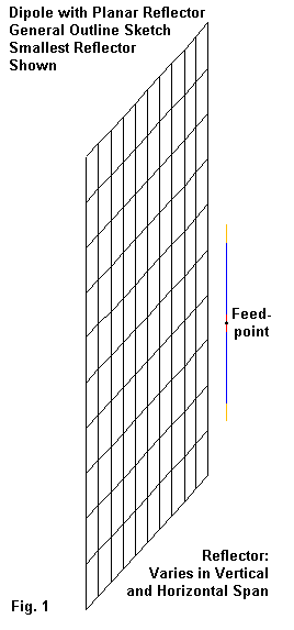
The most basic planar reflector array uses a simple dipole as its driver. For all of the models that we shall explore, the dipole will be vertical, and the entire array will be in free space. Fig. 1 shows the basic outline, tilted in the sketch to show the dipole amid with modeled wires that make up the reflector. The dipole is actually centered both vertically and horizontally relative to the reflector.
For this exercise at 300 MHz, the driver has an 8-mm (0.31") diameter and is 0.436-m long (or 0.436 wavelength). (We shall later see that this diameter is about 1/3rd the effective diameter of the 435-MHz dipole in the earlier article, and this fact will have an effect on the operating bandwidth of the resulting antenna).
The reflector model consists of a standard wire-grid structure using 0.1 wavelength segments with a diameter that is the segment length divided by PI, or about 0.0318 m. Such a structure simulates a tight screen or a solid surface quite well. Since the grid is a parasitic structure, it functions most accurately of all the possible ways in which to use a wire grid. The AGT scores of the models were between 0.997 and 0.998, for only about a 0.01-dB deficit in gain. (Wire-grids function with less adequacy but still well within the usable range when they function as a ground plane to which an antenna is attached, and with least adequacy when the wire grid is part of the antenna itself. The modeling results may still be quite usable, but the modeler needs to pay close attention to adequacy tests the more directly the wire grid is connected to the source.)
Because the reflectors will be used in numerous models of planar arrays, I used the numerical Green's file (NGF) system of incorporating them into models. There are 36 reflectors used in this exercise, each one having a different vertical and horizontal size. The dimensions vary by 0.2 m (0.2 wavelength) in either the vertical or the horizontal dimension from one reflector to the next. The set used here ranges from 1.0 to 2.0 m (1.0 to 2.0 wavelengths) in each dimension. I have coded the models, for example, D-H12-V14 to indicate a dipole driver with a reflector that is 1.2 m horizontally and 1.4 m vertically.
The use of the GM command simplifies reflector construction. I used a central wire, segmented to match the length in 0.1-m increments. Then, 2 GM commands complete the wire collection by replicating the wire enough times to match the opposing dimension. A sample for the H1.2 by V1.4 reflector results in the following NGF file.
CM Planar Reflector 299.7925 MHz (WL=1 m)
CM Y = 1.2 m;  Z = 1.4 m
CM standard wire-grid:  Seg L = 0.1 m; radius = L/PI = 0.0159 m
CM NGF file:  R-H12-V14
CE
GW 1 12 0 -.6 0 0 .6 0 .0159
GM 1 7 0 0 0 0 0 -.1 1 1 1 12
GM 1 7 0 0 0 0 0 .1 1 1 1 12
GW 12 14 0 0 -.7 0 0 .7 .0159
GM 1 6 0 0 0 0 -.1 0 12 1 12 14
GM 1 6 0 0 0 0 .1 0 12 1 12 14
GE 0 -1 0
FR 0 1 0 0 299.7925 1
GN -1
WG R-H12-V14.WGF
EN
See the series on Antenna Modeling for an episode on the rudiments of creating and using numerical Green's files. Since the results of running the model above is only a file of data, we need a second file with the driver, excitation, and output requests. The model corresponding to the reflector just shown and set up for the dipole driver has the following entries.
CM Dipole .175 m from planar reflector
CM Planar Reflector 299.7925 MHz (WL=1 m)
CM Y = 1.2 m;  Z = 1.4 m
CM standard wire-grid:  Seg L = 0.1 m; radius = L/PI = 0.0159 m
CM NGF file:  R-H12-V14
CE
GF 0 R-H12-V14.WGF
GW 24 11 .175 0 -.218 .175 0 .218 .004
GE 0 -1 0
EX 0 24 6 0 1 0
RP 0 361 1 1000 -90 0 1.00000 1.00000
RP 0 1 361 1000 90 0 1.00000 1.00000
EN
The file starts by calling up the data in the stored output of the Green's file. In fact, the reflector portions of all planar arrays will never need to be re-run, since other array models using the reflector need only access the reflector information in storage. Although for small reflectors, we do not save any significant time, for large reflectors, we may save considerable run time.
The dipole (GW 24) is 0.436 m (or wavelength) long with an 8 mm diameter. I have spaced it 0.175 m (or wavelength) in front of the reflector and adjusted its length to provide a feedpoint impedance of 50 Ohms resistive. The currents that it induces in the reflector wire grid appear in Fig. 2.

I have rotated the sketch just slightly to visually offset the dipole so as not to obscure the currents on the wires that it would otherwise hide. I also set the current span from 1E-003 maximum to 1E-017 minimum in order to show relative variations in current levels on the wire grid. Hence, the dipole is uniformly red (the highest current level) since its current exceeds the maximum in the selected range. Blue indicates the lowest current levels.
Because the dipole is vertical, most of the horizontal wire segments in the grid show the lowest current levels. The vertical wire segments show a central region of higher current levels that tapers off as we move away from the positions closest to the dipole. However, there are some values at the reflector edges where we show a slight rise in current relative to what one might think of as an expected progression. The sample shows the smallest reflector used in the exercise, and the patterns are not precisely the same for all reflector sizes. That variation is part of the reason why array performance changes from one reflector size to the next, whether we make the change horizontally or vertically.
E-Plane and H-Plane Performance Variations
One way to sample the performance variations is to examine the free-space patterns of the dipole/planar-reflector array. There are two polar plots of special interest. The E-plane patterns are those taken in a plane parallel to the dipole itself. If the array were over ground, then these patterns would be very close to those azimuth patterns taken with the dipole set horizontally or parallel to the ground surface. The H-plane patterns are taken in a plane at right angles to the dipole. If the array were over ground, then these patterns would be very close to those azimuth patterns taken with the dipole set vertically or at right angles to the ground surface.

Fig. 3 shows some selected E-plane patterns illustrating the evolution of the pattern across the span of sampled reflectors. The upper left pattern with 3 large rear lobes is typical of reflector sizes that are smaller than or equal to, in any progression, the size needed for maximum gain. As the reflector size increases past the size needed for maximum gain, the rear lobes shrink to the ones shown in the upper right pattern. Note the emergence of two added lobes. If we continue the progression to larger reflector sizes, the 180-degree rearward lobe disappears, as shown in the lower left pattern. In the lower right pattern, we see the highest 180-degree front-to-back ratio, created by a deep null to the rear of the heading for maximum gain. However, note that once we pass the reflector size needed for maximum gain, the worst-case front-to-back ratio remains relatively constant in the 22-24-dB range.

In Fig. 4, we have a progression of H-plane patterns. The wider beamwidth results from the fact that these patterns are at right angles to the dipole. Not every progression shows all of the shapes indicated in the drawing, but once more, they show a sort of averaged evolution. The smallest reflectors vertically tend to begin with an inverted pear shape pattern, as shown in the upper left. The pattern tends to evolve with increases in the vertical dimension to a more squared rear lobe structure, as illustrated at the upper right. Maximum front-to-back ratio for any progression of the vertical dimension tends to end with the nearly cardioidal pattern at the lower left, with only a rain drop for a rearward lobe. However, as we increase the horizontal dimension, we encounter a widening of the H-plane beamwidth. At the widest and tallest reflector sizes, the forward lobe begins to split. The forward-line null created by the split is never great (about 0.3 dB maximum), but is apparent in the lower right pattern.
We can follow the pattern data by also viewing the E-plane and the H-plane -3 dB (half-power point) beamwidths. Fig. 5 shows the progression of beamwidths for the E-plane patterns. In this and subsequent data graphs, I have somewhat arbitrarily placed the horizontal reflector dimension increments into separate lines, while using the X-axis for the increments of the vertical dimension. One could reverse the convention, but the data would not change.

The range of variation among all of the data for all reflectors is small for the E-plane beamwidth. There are two main clusters of lines because the data appears as integers with 1 degree each side of the centerline being the minimum. Hence, the beamwidth changes in steps of 2 degrees. Only as we increase the vertical dimension of the reflector to and beyond 1.8 m (or wavelength) do we obtain distinct values for most of the horizontal sizes.
However, note that as we increase the reflector size vertically, we obtain a minimum beamwidth value at a reflector height of 1.2 m (or wavelength). Minimum E-plane beamwidth tends to coincide with maximum gain and increases regularly beyond that point.

H-plane beamwidth, graphed in Fig. 6, shows a similar correspondence between maximum gain and minimum beamwidth, at least until we reach to two widest horizontal dimensions. The horizontally smaller reflectors also show another interesting feature: beyond a certain vertical height, the H-plane beamwidth remains constant. The two horizontally largest reflector change the progression by showing a continued increase in beamwidth as we increase the vertical dimension of the reflector. These are precisely the reflector dimensions that also show the beginnings of a split in the forward lobe.
Resistance, Reactance, Gain, and Front-to-Back Ratio
The reflector size may undergo a 4:1 variation in area (from 1.0 m by 1.0 m to 2.0 m by 2.0 m) without requiring any change either in the length of the driver or its spacing from the reflector. As the sample model showed, the driver remains at a spacing of 0.175 m from the reflector throughout the exercise. The highest SWR encountered at the design frequency was 1.03:1.

Fig. 7 shows a composite of the SWR curves for the smallest and the largest reflectors, along with the curve for the situation yielding the highest gain. The three curves are so coincident that the individual lines are indistinguishable. The 2:1 SWR passband is about 29-30 MHz or about 10% of the design frequency. The limited SWR passband results in part from the 8 mm (0.31") diameter dipole. One can easily expand the SWR passband by increasing the element diameter. In the earlier article, I used a 0.5" element at 435 MHz, which is electrically about 2.3 times fatter than the one used in this exercise. The result was an SWR curve under 1.5:1 across all of the 70-cm amateur band. The length of that fatter element was 0.416 wavelength, compared to 0.436 wavelength for the dipole used in this exercise. The thickness of the dipole driver--once brought to a 50-Ohm resonance--has virtually no affect upon array performance.

Although Fig. 8 may seem to present a jumble of lines, it actually shows some interesting facets of the behavior of the feedpoint resistance as we change the reflector size. The narrowest reflectors horizontally tend to have marginally higher feedpoint resistance values than the widest reflectors. Feedpoint resistance is not a strict function of gain, as was the E-plane and H-plane beamwidths. The minimum feedpoint resistance values occur one to two increments of vertical reflector height beyond the maximum gain dimension.

Reactance values more closely parallel gain performance, with all horizontal widths showing the maximum capacitive reactance at the vertical dimension that corresponds to maximum gain. Only the widest reflector (2.0 m horizontally) shows a small variation from this pattern. As well, the reduction in the capacitive reactance is not a constant curve as we increase the vertical dimension of the reflector. Note that all of the reactance values show a slight increase in capacitive reactance as the reflector reaches its maximum vertical length (20 m for this exercise). However, the variations in both the feedpoint resistance and the feedpoint reactance would be difficult to measure under the best circumstances. In both cases, the maximum variation is only a bit over 1 Ohm.
I have reserved the gain and front-to-back data for last. My goal has not been to create suspense, but rather to enforce attention to facets of array behavior that we often overlook in our haste to encapusulate array performance in one or two figures. However, the time has come to examine the array gain using a dipole with varying sizes of reflectors.

The curves in Fig. 10 parallel each other, except for the minor deviations of the curve for the smallest reflector. For maximum gain, there is a numerically clear winner: the reflector having a vertical dimension of 1.2 m and a horizontal dimension of 1.2 m. With this reflector, the modeled free-space gain is 9.31 dBi, about the same value as a long-boom 4-element Yagi. However, note that the reflectors one step smaller and one step larger approach this value so that there would not be an operationally detectable difference. Hence, we might wish to withhold our declaration of the "winner" for a moment.
Note that as we increase the horizontal dimension beyond about 1.4 m (or wavelength), gain decreases with any size reflector vertically. As well, as we increase the vertical dimension beyond 1.2 m (or wavelength) the gain also decreases. The gain never decreases to below the level of a long-boom 3-element Yagi, but the decrease from peak value is clearly evident.

The 180-degree front-to-back ratio curves in Fig. 11 demonstrate why I suggested withholding a declaration of a winning reflector size. Most evident is the fact that the narrower reflectors show the highest 180-degree front-to-back ratios when combined with the tallest vertical dimension. However, review the E-plane patterns in Fig. 3, with special attention to lower right pattern. Although the 180-degree front-to-back ratio is very high (nearly 31 dB), the worst case front-to-back value is no different from the other patterns (about 22-24 dB).
Except for the widest reflectors, there is a general trend toward higher front-to-back ratios with increasing reflector height. The values at the height of maximum gain (1.2 m vertically) tend to be lower due to the prominent 3-lobe rear structure of the pattern, also shown in Fig. 3. However, as we increase the horizontal dimension at the maximum gain vertical dimension, the front-to-back ratio tends to increase. With a horizontal dimension of 1.6 m and a vertical dimension of 1.2 m, we lose only 0.17 dB of forward gain, but arrive at a front-to-back ratio over 20 dB.
Changing the Dipole Diameter and Spacing
I have noted in passing that changing the diameter of the dipole in front of the planar reflector will have little effect on array properties other than to change the 50-Ohm 2:1 SWR passband. Although this assertion may seem intuitively obvious, we should check it. The process only requires that we alter the dipole in selected models in order to bring it to resonance at the test frequency (299.7925 MHz).
Since there is a reflector that yields a distinct gain peak (H = 1.2 m, V = 1.2 m), we may use this model as a first-order check to see if the claim is confirmed or refuted. I simply took the model for this reflector and applied it to both the original dipole and two replacements. Of course, changing the dipole diameter required changing its length. As well, the process required very small changes in the spacing between the reflector and the dipole.
The following table shows the resulting dimensions and performance reports from the exercise.
Dipole          Dipole      Space from      Free-Space     Front-to-Back     Impedance        50-Ohm
Diameter        Length      Reflector       Gain dBi       Ratio dB          R +/- jX Ohms    SWR
 8 mm (0.31")   0.436 m     0.175 m         9.31           18.33             49.44 - j1.25    1.03
16 mm (0.63")   0.422 m     0.176 m         9.30           18.29             49.45 + j1.09    1.02
24 mm (0.94")   0.412 m     0.177 m         9.31           18.24             49.32 - j0.91    1.02
As with all dimensions in meters in this exercise, a length in meters is also a length in terms of a wavelength. Hence, scaling to a desired frequency is simplified. As predicted, the change in diameter over a 3:1 diameter ratio yields no significant change in performance. The 50-Ohm SWR curves in Fig. 12 are equally revealing.

Obviously, the fatter the dipole, the broader the SWR curve. The 8-mm diameter dipole shows a 2:1 SWR between about 287 and 316 MHz, or a 9.7% passband. Doubling the diameter to 16 mm increases the lower and upper limits to about 284 and 319 MHz, respectively, for an 11.7% passband. A further increase to 24 mm sets the limits at 282 and 232 MHz, for a 13.7% passband. In critical applications, a fatter dipole may indeed be advantageous.
If we scale the dipoles for the 70-cm band, the smallest diameter dipole would be between 3/16" and 1/4". The mid-sized dipole would be equivalent to about 7/16", and the fattest dipole modeled would be just over 5/8". You may divide these values by 2 and by 3 for rough diameters serving 903 and 1296 MHz.
A second premise of this study has been that the designer will normally select the element spacing from the reflector to arrive at a convenient or target feedpoint impedance. Given that amateur practice tends to focus upon 50-Ohm coaxial cables, I used 50-Ohms as the study target.
The spacing of the driver from the reflector does tend to control two factors: the gain for a given reflector size and the feedpoint impedance. To bring the driver to resonance for any given spacing will be a necessary step in redesigning for an alternative feedpoint impedance. The following table provides data on three sample reflector-to-driver spacings for our simple dipole array. The reflector used for the samples was the smallest of the lot (1.0 m by 1.0 m). The driver is 8-mm in diameter throughout.
Reflector-to-      Element     Free-Space     Front-to-Back     Impedance
Driver Space       Length      Gain dBi       Ratio dB          R +/- jX Ohms
0.135 m (wl)       0.438 m     9.05           17.78             33.02 - j0.99
0.175 m (wl)       0.436 m     8.86           17.31             49.85 - j0.24
0.25 m (wl)        0.444 m     8.31           15.94             80.44 + j0.89
The gain and the 180-degree front-to-back ratio tend to increase with closer spacing between the reflector and the driver. Conversely, both values tend to decrease with wider spacing. When starting this study, I decided that the gain increase with closer spacing was not sufficient to warrant a requirement for a complex matching system. However, some of the more complex driver systems yet to be explored may require a wider spacing to obtain a desired feedpoint impedance, suggesting that we may not derive all of the possible gain from them. With the home antenna builder in mind, I have accepted this imperfection to focus on designs that one might produce as physical antennas with some ease.
Conclusions So Far
Our exploration of a simple dipole placed in front of a planar reflector has produced a number of interesting results.
1. Although the feedpoint resistance and reactance show some interesting data curves, the range of variation is so small as to allow the conclusion that the feedpoint impedance does not change materially with changes in reflector size.
2. The SWR passband is a function of the driver diameter and not a function of the reflector size.
3. For maximum gain, there is an ideal reflector size, namely 1.2-m (wavelength) by 1.2 m (wavelength). Horizontal variations from 1.0 m to 1.6 m show only a small reduction in gain, although variations in the vertical dimension show more evident gain reductions.
4. The larger the horizontal dimension, the higher the initial front-to-back ratio with the smaller vertical dimensions. However, a 20-dB front-to-back ratio is easily achieved at the ideal vertical dimension of 1.2 m (wavelength), with a horizontal dimension of 1.6 m (wavelength). Still, with the ideal horizontal dimension for maximum gain (1.2 m or wavelength), the front-to-back ratio is well above 18 dB.
This summary does not tell the complete story in the data, but it hits the most essential points. A simple dipole in front of a planar reflector--whether solid or a screen to slip the wind--constitutes a very useful and buildable utility antenna for the UHF range, especially. But the exercise does leave us in a quandary.
If we change the type of driver that we use for the array, will the ideal reflector size also change? Some drivers, such as a pair of dipoles in phase or a rectangle, have multiple vertical elements that are not centered. Will they need a full 0.6 m (wavelength) spacing of reflector beyond the outer driver edge to achieve maximum gain? Will such drivers show greater or lesser coincidence between the ideal reflector size for gain and front-to-back ratio? Will these drivers be equally insensitive to reflector size with respect to the feedpoint impedance?
It looks like I'll have further use for those reflectors whose data is stored in Green's files.
How Reliable Are These Models Relative to Their Purpose?
The models used in this exercise are designed to provide general guidance relative to the performance trends of planar reflector arrays. They are not designed to provide specific design parameters for a physical antenna. Design-specific models would require prototypes using the intended construction methods to confirm or modify the generalized features of the models.
However, even in the realm of providing general guidance, we may distinguish between two types of conclusions drawn from the data collected from the models. The first type of conclusion focuses upon the general trends in performance as we change the size of the reflector. These conclusions are likely to be quite accurate. The second type of conclusion identifies specific reflector sizes for peak (or null) performance in some category or another. These conclusions are subject to variation within some yet to be specified range.
There are tests that are relevant to the type of project being conducted, tests that we can perform within the context of modeling. In the present case, we may construct a series of reflectors using a much closer spacing of the wire-grid elements. The changes of performance reports or the changes that we may need to make in the model to achieve a given target performance can provide an indication of how much a physical antenna may vary from the models. The normal procedure would be to use a much more dense wire-grid, perhaps twice as dense as the standard wire-grid structure. Since the original models used wire-grid segment 0.1 m long, with a radius of 0.0159 m, we can rebuild the reflectors using segment lengths that are 0.05 m long with a radius of 0.008 m. The process also facilitates reflector growth in 0.1-m steps, allowing the modeler to refine certain judgments concerning what size reflector yields a certain peak performance value.
To test the present models, I constructed denser reflector wire-grids for the region surrounding the peak forward gain report. That report identified a 1.2-m vertical dimension and a 1.2-m horizontal dimension as the peak free-space forward gain size, using 0.2-m increments between steps. Therefore, I constructed denser reflectors with vertical dimensions that ran from 1.1 m to 1.3 m, with horizontal dimensions between 1.1 m and 1.5 m. Although the reflectors vary from the originals, the driver (dipole) itself remains unchanged: 0.436 m long with an 8-mm diameter and spaced 0.175-m from the reflector.
Since the data covers only a limited span of the total covered in the initial model sweeps, we may survey it in tabular form. In this instance, the table has 3 sections, separated by the levels of the reflector's vertical length. Each data grouping within a section proceeds according to increases in the horizontal length of the reflector.
Vertical = 1.1 m
Horizontal    Free-Space    Front-to-Back    E-BW       H-BW       Impedance        50-Ohm
Length        Gain dBi      Ratio dB         degrees    degrees    R +/- jX Ohms    SWR
1.1 m         9.05          17.96            56         82         49.77 - j0,92    1.02
1.2 m         9.09          18.39            56         82         49.70 - j1.01    1.02
1.3 m         9.11          18.90            56         82         49.62 - j1.04    1.02
1.4 m         9.09          19.49            56         82         49.56 - j1.09    1.02
1.5 m         9.06          20.16            56         84         49.53 - j1.01    1.02
Vertical = 1.2 m
Horizontal    Free-Space    Front-to-Back    E-BW       H-BW       Impedance        50-Ohm
Length        Gain dBi      Ratio dB         degrees    degrees    R +/- jX Ohms    SWR
1.1 m         9.22          18.17            54         82         49.53 - j1.29    1.03
1.2 m         9.26          18.45            54         80         49.44 - j1.36    1.03
1.3 m         9.27          18.82            54         82         49.35 - j1.36    1.03
1.4 m         9.25          19.28            54         82         49.28 - j1.33    1.03
1.5 m         9.20          19.85            54         84         49.25 - j1.27    1.03
Vertical = 1.3 m
Horizontal    Free-Space    Front-to-Back    E-BW       H-BW       Impedance        50-Ohm
Length        Gain dBi      Ratio dB         degrees    degrees    R +/- jX Ohms    SWR
1.1 m         9.30          18.85            54         82         49.17 - j1.38    1.03
1.2 m         9.32          18.93            54         82         49.09 - j1.42    1.03
1.3 m         9.32          19.11            54         82         49.01 - j1.40    1.04
1.4 m         9.29          19.41            54         84         48.97 - j1.35    1.03
1.5 m         9.23          19.84            54         84         48.96 - j1.30    1.03
The data cover in more detail a much smaller span of reflector variations, so the small variations from step to step are natural. For example, the E-plane and H-plane beamwidths vary by only 2 degrees in either plane across the entire set of models.
The denser grid structure suggests that both vertical and horizontal reflector dimensions of 1.3 m (wavelength) are closer to the precise dimensions for maximum overall gain from the planar reflector array using a single dipole driver. The 0.2-m increment used in the initial modeling could not have revealed such a result. We may also note that a horizontal dimension of 1.2-m (wavelength) also yields the reported 9.32-dBi maximum gain value.
The two points within the table that correlate to points of our original grid dimensions use horizontal dimensions of 1.2 m and 1.4 m with a vertical height of 1.2 m. In both cases, the denser grid yields gain values that are lower than the original, but only by 0.02 to 0.05 dB. The 180-degree front-to-back ratios also differ for the two points, both being up by about 0.1 dB. The resistance values are the same, with a reactance variation of only about 0.1 Ohm. Both E-plane and H-plane patterns would overlay each other to hide one beneath the other.
The results of this test--although limited to a small span of array sizes--suggest that the 0.1 wavelength per segment wire grid is quite reliable as a simulation of either a tightly-spaced screen or of a continuous surface. Indeed, one of the reasons for using fairly large diameter wire in the grid is to achieve the effect of a solid surface. The internally available tests of the initial models suggest that the numerical results with respect to gain and front-to-back are good to the first decimal place. As well, one may have good confidence in the features of the E-plane and H-plane patterns.
Our future episodes in this saga will use the wider spacing of grid wires throughout for consistency and ease of data gathering. As we halve the length of each segment within a grid of constant perimeter dimensions, the number of segments expands by a factor of nearly 4. Hence, it is possible to exceed the capabilities either of the core or of one's patience. Nevertheless, before we have reached the end of the final episode in this series, we shall again return to the question of model reliability. As well, nothing in the confidence that the test yields for the models is a substitute for careful prototype construction and measurement.
Updated 02-01-2005. © L. B. Cebik, W4RNL. This item originally appeared in antenneX January, 2005. Data may be used for personal purposes, but may not be reproduced for publication in print or any other medium without permission of the author.