Let's begin with notes on two antenna concepts that meet in these notes.
1. From about June, 2001 through November, 2002, Dan Handelsman and David Jefferies presented a series of articles in antenneX on an interesting concept in broadband antennas: the prismatic polyhedron. Dan eventually patented the idea. Some of the versions were capable of 3:1 frequency ranges with a 2:1 SWR or under at the listed antenna impedance. (In bandwidth percentage terms, a 3:1 frequency range translates into a 100% bandwidth.) Some of the relevant articles and their links are the following:
"Plate Dipoles and Prismatics," by Dan Handelsman and David Jefferies
(http://www.antennex.com/archive5/Apr02/Apr402/pdp.html : No copy on web.archive.org - page required login)"Plate Dipoles and Prismatics Revisited," by David J. Jefferies and Dan Handelsman
(http://www.antennex.com/archive5/May02/May402/pdp2.html : No copy on web.archive.org - page required login)"Prismatic Polyhedron Antenna Measurements at Low GHz Frequencies," by David J. Jefferies
(http://www.antennex.com/archive5/Nov02/Nov502/pms.html : No copy on web.archive.org - page required login)"Cage Dipoles and the Prismatics," by Dan Handelsman and David Jefferies
(http://www.antennex.com/archive5/Dec02/Dec402/cage.html : No copy on web.archive.org - page required login)
The third item contain links to further articles on the broadband antenna.
2. Some time back I published a series of articles on planar and corner reflector arrays that resulted in a book of the same title (Planar and Corner Reflector Arrays, available from antenneX). A planar reflector is a solid sheet, screen, or curtain of wires or rods, optimally sized for the driver and spaced to achieve the best compromise between gain and the feedpoint impedance. Almost all of the modeled drivers increased their SWR and operating bandwidths when used with a planar reflector. In each case, the bandwidth increase occurred mostly on the high side of the design frequency. However, the SWR bandwidths were generally less than about 10% relative to the center or design frequency.
However, a pair of dipoles spaced 1/2 wavelength and fed in phase achieved an SWR bandwidth of about 26% (about 75 MHz at a center frequency of 300 MHz) while retaining its pattern shape and other operating characteristics. A batwing dipole formed a contrast to the phased dipole pair. An independent batwing shows an SWR bandwidth of over 50% (about 150 MHz at a center frequency of 300 MHz). When provided with a planar reflector, the bandwidth dropped to about 33%, that is, it showed a loss of about 50 MHz. The two wide-band designs left open a number of questions, some specific to the driver types and some generic to the use of planar reflectors.
The most fundamental question in the present context concerns the useful frequency range for a given planar reflector. Planar reflectors with ordinary drivers having modest bandwidths showed remarkably stable operating characteristics across the SWR bandwidths. However, none of the drivers stressed either the spacing between the driver and the reflector or the reflector size within the limits of operation. Hence, none of the drivers provided data on the potential limits of a planar reflector.
David Jefferies recently called my attention to the prismatic polyhedrons, and so I decided to explore at least some of these very wide-band antennas in the context of creating a directional array using a planar reflector. The results so far have proven to be interesting and possibly general.
The P3 Antenna
Most of these notes employ one of Dan Handelsman's designs, the P3 cut for a lower limit of about 300 MHz. Fig. 1 shows the outline of the antenna and includes dots to indicate segmentation of the wires. The P3 consists of 3 dipoles, each center fed, with triangular junctions at the outer ends. Unlike a cage dipole, where we draw the cage to a center feedpoint, the P3 uses continuous elements. From the center of each element to a central feedpoint, we employ short transmission lines, all the same length and impedance. Thus, we end up with three dipoles fed in phase with relatively close spacing and connected outer ends.

The test antenna replicated one of the existing designs. The wires are all 0.015 m (1.5 cm) in diameter. Fatter wires increase the operating bandwidth, but the requirements of modeling limit the usable wire diameter. Since the antenna has corners, some as narrow as 60 degrees, using too fat a wire places the surface of one wire within the center region of an adjacent wire segment, a situation that results in NEC warning or error messages. The modeled antenna height (or the length of each long wire) is 0.32 m. Each face (or top/bottom wire) is 0.083 m. The transmission lines from the dipole centers to the common feedpoint are each 300 Ohms, and with a velocity factor of 1.0, the length is 0.05 m. All modeling for the P3 and subsequent arrays used free-space as the environment.
The modeled P3 showed a 50-Ohm SWR curve with approximate limits of 300 and 760 MHz, for better than a 2.5:1 frequency ratio or about an 87% bandwidth. Dan achieved slightly better results by judicious model tweaking, while some lab versions of the antenna tested by David showed a measured frequency range of more than 3:1. However, for our inquiry, the 2.5:1 range is more than satisfactory. Fig. 2 graphs the progression of feedpoint resistance and reactance, as well as the 50-Ohm SWR across the swept passband. The resistance and reactance values vary over small ranges and undulate, resulting in a wide SWR curve with two low points (similar to the SWR curves of paired driver-first-director elements in an OWA Yagi).

The wide SWR bandwidth of the P3 does not result solely from the antenna geometry. The selection of the phase-line Zo and length also help to shape the SWR curve and the impedance to which we reference the SWR.
Table 1 lists the reported data for the P3 as an independent antenna. The table uses 100-MHz increments from 300 through 800 MHz as sampling points. The left-most columns show the growth of the antenna across the sampling range when we measure the elements in terms of wavelengths.

You may correlate the impedance data in the table to the information in Fig. 2. However, the table includes other significant information for those wishing to model the P3 and similar antenna. The column labeled AGT provides the NEC-4 AGT score for the antenna at each sampled frequency. The adjacent column lists the amount by which to decrease the reported gain to arrive at a more accurate figure. Since we are looking for relatively gross trends, corrections less than 0.1 dB in the gain and 2% or less in the feed resistance column are not significant. (In other modeling exercises, they might become important.)
As we increase the frequency of operation without altering the physical structure of the P3, we note an increase in the free-space gain. By 800 MHz, the gain has risen almost 1.3 dB. Fig. 3 provides an indications of why this occurs. As the frequency increases, the E-plane (or elevation, given that the model stretched along the Z-axis) patterns show a decreasing beamwidth. (The H-plane or azimuth patterns would show simple circles, so I omitted them.) Between any two adjacent patterns, the change is hardly noticeable, but if we compare the 300-MHz and the 800-MHz patterns, the elevation "squeeze" in the pattern is readily evident.

The triangular P3 would serve well as either a horizontal or a vertical dipole, especially in UHF applications. Since the SWR bandwidth does vary with the diameter of the wires composing the structure, its use in HF applications, where wires are very thin (relatively speaking), is uncertain, although Dan has addressed such uses in some of his articles. At 30 MHz, the triangle face would be 0.83 m, and at 3 MHz, it would be 8.3 m. These values, of course, rest on also scaling the wire diameter to .15 m at 30 MHz and to 1.5 m at 3 MHz. Fortunately for our goals in these notes, we may simply use the model that we have described.
The P3 with a Planar Reflector
Providing the P3 with a planar reflector is, in principle, a relatively straightforward project. Extensive modeling with many types of antennas--ranging from lower HF NVIS aerials to UHF arrays--has yielded a rough rule of thumb. For maximum gain and a good front-to-back ratio, the reflector should extend beyond the limits of the antenna by between 0.45 and 0.55 wavelength in both planes. Therefore, the initial reflector had a size of 1.0 m side-to-side across the face of the P3. The reflector height used was 1.2 m.
A wire-grid rectangle will generally simulate a solid surface if its wires are no longer than 0.1 wavelength between junctions. To achieve the solid-surface simulation, each wire must have a diameter determined by dividing the wire length between junctions by PI. However, we must introduce a caution here. Make the calculations at the highest frequency to be used. Using a lower frequency may result in a leaky grid or one in which the wires approach resonance. For our very wide-band project, the caution is very significant. Using 800 MHz as the wire-grid construction frequency results in models with many more segments, in some cases approaching 2000. Serious modelers should consider investing in advanced software if their entry-level packages have lower segment limits.

Fig. 4 shows the outline of the P3 and reflector as modeled. Note that two long legs of the P3 are equidistant from the reflector, while the third leg is about 0.07 m farther forward. I selected a spacing between the driver and the reflector that results in the best compromise between the impedance and the pattern performance. The final value was 0.2 m. Table 2 shows the distance in wavelengths for each of our sampling frequencies. Note that at 800 MHz, the spacing has grown to over 1/2 wavelength. Most designers of wide-band HF dipole curtain arrays use a design-frequency spacing of about 0.3 wavelength. The test array reaches this level before the frequency increases to 500 MHz.

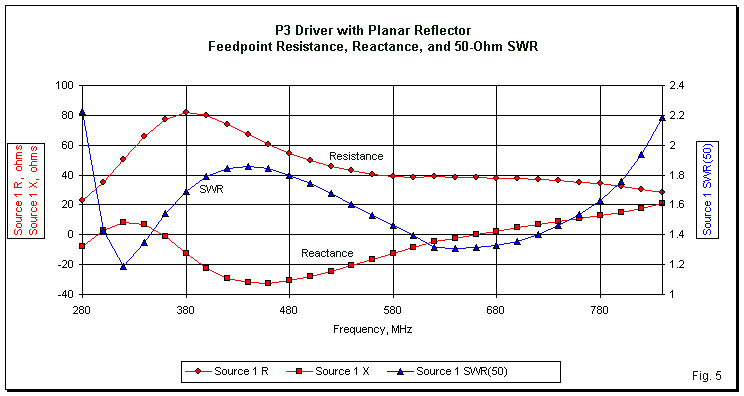
The selected spacing does not yield the best possible impedance curve. A spacing of 0.22-m is slightly better, but at a cost in other performance categories. Fig. 5 shows the resistance, reactance, and 50-Ohm SWR using the selected spacing between the driver and the reflector. The 2:1 SWR bandwidth has increased its range to 285-820 MHz. The increase is about 15 MHz on the low end, but 60 MHz at the upper end of the range--compared to the independent P3. A single graph of impedance performance is sufficient for all of the models that we shall use. Although we shall vary some of the reflector dimensions, the spacing between the driver and the reflector will not change. As a result, the feedpoint impedance values do not change by more than very small amounts that we may track in the data tables. For any given planar reflector array, the driver feedpoint impedance is relatively insensitive to changes in the size of the reflector.
Adding the large planar reflector has increased the SWR bandwidth of the P3. However, we do not yet know if the increase is worthwhile in terms of the radiation patterns produced by the antenna. One way to present such data might be to use a frequency sweep curve. Unfortunately, such curves become very misleading if the maximum gain happens to occur at an angle other than the bore sight of the antenna. In such cases, recorded 180-degree front-to-back ratio values will reference the maximum gain heading. Hence, they will not give a true indication of the direct rearward performance of the array. For this reason, we shall explore the performance of the P3+reflector by using both tables and galleries of patterns, each at successive 100-MHz sampling steps. The front-to-back value shown in the table will be the ratio of maximum gain to a direction tangent to the rear of the planar reflector. Table 3 provides our first overdose of data.

The table has 4 types of entries. Regular type indicates that a pattern is normal, with a forward lobe and only smaller rearward radiation pattern structures. Italic type points to patterns with a single large forward lobe, but with two main headings, each equally off the axis of the array. Boldface entries indicate that the main lobe has split into two lobes, each off axis by the same amount but on opposite sides of the bore sight line. What distinguishes a two-lobe pattern from one with two main headings is the fact that each main lobe has its own beamwidth. In other words, the null between lobes is greater than 3 dB. Finally, entries that are both bold and italic indicate the presence of three distinct lobes, each of which is very significant.
You may best examine the tabular data in conjunction with an associated gallery of H-plane (azimuth) patterns. For our initial, seemingly optimal reflector size, the patterns appear in Fig. 6. Note that for large reflector, only the pattern for 300 MHz is perfectly well behaved, that is, having a single forward and a single rearward lobe. At 400 MHz, the main lobe already shows two main bearings, with a slight decrease in gain along the main axis of the array.

The remaining patterns in Fig. 6 provide a fairly good commentary on lobe splitting and widening and on the development of increasing numbers of forward lobes. Interestingly, the rearward lobe remains singular and quite weak. The general conclusion that one might reach is that for the P3, a large or full-size reflector limits the effective operation of the P3 to somewhere between 400 and 500 MHz, despite the fact that the SWR bandwidth is much wider.
At this stage, the potential for improvement is limited. We cannot change the spacing from the reflector to better optimize that spacing at higher frequencies without radically altering the SWR curve. To restore the SWR curve--assuming that it is amenable to restoration--would require considerable redesign of the P3 itself. Numerous flatter drivers have quite different dimensions when optimized for planar reflector use than we find when we use the driver as an independent antenna.
If we retain the given dimensions of the P3--which we shall do--then we have only one significant option: to change the size of the reflector. Spot checks of the model suggested that below the design limit (about 300 MHz at the low end of the passband), the patterns remain well behaved, even though the feedpoint impedances are not usable. The suggestive consequence of these checks is that we might widen the operating passband with improved pattern shapes if we reduce the size of the reflector. Rather than using a series of slow steps, I simply halved the reflector size to 0.5 m in the H-plane (horizontally) and 0.6 m in the E-plane (vertically). Again, I set the wire-grid dimensions at 800 MHz to ensure a structure that would not resonate at some intermediate frequency. Table 4 and the gallery of H-plane patterns in Fig. 7 provide the results of this modeling experiment.


In one sense, the experiment is a success, since patterns are quite normal through 600 MHz. Even though the 500-MHz pattern is technically a dual-heading plot, the decrease in gain along the array main axis is insufficient to make the antenna less than fully functional. However, the patterns show a considerable reduction of gain. At 300 MHz, the gain is down by 1.5 dB compared to the value with the large reflector.
In addition, the rearward radiation structure shows considerably greater development with the smaller reflector, resulting in somewhat mediocre front-to-back values. The beamwidth of the rearward lobe is much greater than for the rearward lobe with the full-size reflector. Perhaps the single relatively stable dimension of performance lies in the feedpoint impedance. If you compare the Feed R and Feed X values in Table 3 and in Table 4, you will find only relatively insignificant differences. The 2:1 50-Ohm SWR bandwidth still extends from 285 to 820 MHz.
The data make clear that finding a compromise reflector size is one key to extending the performance of the P3 driver. However, the required reduction in reflector size results in degraded performance relative to both forward and rearward radiation. The limit of what we might call (without criteria to impose a definition) "adequate" performance is perhaps 550 MHz at most. This somewhat arbitrary limit frequency value results in a frequency range that is less than 2:1 (although it is wider than the best obtained for the batwing antenna as a driver). The bandwidth in percentage terms is under 60%.
Past studies of planar reflectors indicate that for the normal range of driver assemblies (all 2-dimensional), variations of reflector dimensions did not equally affect both the forward gain and the front-to-back ratio. Peak gain occurs at a reflector size that is below the optimal E-plane (vertical) dimension that yields the best front-to-back ratio. Both dimensions contribute to the front-to-back ratio, but the vertical dimensions seemed more pronounced in its effect. Whether we can make a similar differentiation with the P3 is an interesting question. Therefore, let's begin again with the large reflector (Table 3) and see what results from changing only one of the dimensions at a time.
Table 5 and the gallery of patterns in Fig. 8 supply the results of shrinking only the H-plane or horizontal dimension to 0.8-m. The vertical dimension remains at 1.2-m.


Except for the gain at 300 MHz, the reduction in reflector width appears to have yielded an improvement. The first appearance of dual headings is at 500 MHz (instead of 400 MHz, as in the original reflector exercise). In addition, the front-to-back ratio remains universally good, and the rearward patterns remain small and distinct. However, from somewhere just below 500 MHz upward in frequency, the patterns become unusable, if the goal is maximum gain on a forward direction.
We may repeat the experiment, this time reducing the vertical dimension to 0.9-m. The horizontal dimensions returns to its original 1.0-m value. The results of this experiment appear in Table 6 and in Fig. 9.. One conclusion that we can draw from both new experiments is that the impedance values are well within the range of those resulting from the use of the full-size large reflector and from the small reflector. Since we did not change the spacing between the P3 and the reflector surface, the 2:1 50-Ohm SWR range is still 285 to 820 MHz.


The results of the experiment are complex when we make multiple comparisons. The gain values at the lower end of the spectrum are lower than for either of the two comparators just discussed. However, the pattern at 400 MHz has more gain than the pattern with a shrunken horizontal dimension. Despite this apparent improvement, the table shows that the 500 MHz pattern introduces a double forward heading just as did the pattern with a reduced horizontal dimension. As well, the forward lobes above 500 MHz are split to roughly the same degree.
The effect of the vertical dimension reduction in the reflector on the rearward pattern is less a matter of numbers than of structure. The shape of the rearward pattern at 300 and 400 MHz is somewhat of a teardrop, rather than the distinct rearward lobe that we obtained from reducing the horizontal dimension of the reflector. Although the 180-degree values remain reasonably good for a planar reflector array, the rearward lobes have taken on a more complex form at higher frequencies. In general, the rearward patterns show a greater beamwidth than did the rearward patterns created by shrinking only the horizontal dimension.
Both experimental intermediate reductions in reflector dimensions fall short of extending the operating range of the array to the extent of the half-size reflector. However, they do indicate directions for experimentation, depending upon the limits of gain reduction and the limits of rearward performance reduction that we bring to the experiment. Each intermediate dimension reduction extended the operating range by at least 100 MHz over the full-size reflector. However, the small reflector extended the range well past 500 MHz--but with further performance reductions. What compromise is best for a potential application depends upon the project requirement we bring to any further modeling.
In addition, these notes have restricted themselves to strict planar reflectors. Hence, they provide no clue to what might occur with the use of a corner reflector or a parabolic reflector.
The P2 without and with a Planar Reflector
I purposely began with the 3-dimensional driver in order to evaluate its potential for use in a planar reflector array. The P3 has only 2 elements that are 0.2 m from the reflector. The third element is another 0.07 m farther away. Given the fact that a change of as little as 0.002 m could change the array's SWR curve, we likely should not underestimate the consequences of placing a 3-dimensional driver array in front of a planar reflector.
One way to perform a quick check on the difference between a 2-D and a 3-D driver is to perform at least a perfunctory evaluation of the P2 antenna. The P2 forms a rectangle. In our application, the long legs are 0.356 m, while the short sides are 0.075 m. The wire diameter is 0.015 m (1.5 cm). Using Dan's formulations as a guide, I aimed for a feedpoint impedance centered on 75 Ohms. As shown in Fig. 10, the central feedpoint required two transmission lines, each with a characteristic impedance of 280 Ohms. Each line, with a velocity factor of 1.0, is 0.06 m long.

As Fig. 11 reveals, the SWR behavior referenced to 75 Ohms is not quite as neat as for the P3. Nor is the 2:1 SWR bandwidth as great. The range for the P2 is 305 to 760 Ohms, very slightly less than for the P3. Nevertheless, the shapes of the resistance and the reactance curves are very close to those that we saw with the independent P3; only the values differ.

Table 7 summarizes the data for the P2, beginning with the dimensions given in wavelengths at each sampled frequency. To the right are the AGT scores and the required correction of the raw gain reports. Due to the relative simplicity of the P2 structure, these values are superior to the values we obtained for the P3.

The P2 gain values require some explanation. At first sight, they appear to be universally higher than the gain values obtained for the P2. However, the P3 develops an essentially circular H-plane (azimuth) pattern. The P2 does not. Since P2 consists of two dipoles fed in phase with a small space between, the broadside gain is higher than the edgewise gain. The amount of broadside-to-edgewise difference increases with frequency, since the face distance also increases with frequency. The gallery of free-space H-plane patterns appears in Fig. 12. The gallery omits the elevation or E-plane patterns since these are so similar to the ones we saw in connection with P3 in Fig. 3. In general, averaging the maximum and the minimum gain for each patterns yields a value similar to the corresponding P3 gain value at each sampled frequency.

For the purposes of comparison, I created only a single planar reflector using the small dimensions that produced the most extended operation of the P3 driver. The reflector is 0.5 m horizontally by 0.6 m vertically. The P2 is 0.2 m ahead of the reflector, the same spacing used for the P3. However, the P2 driver proved to be not as well behaved as the P3. It required a change in both the Zo and the length of the phase lines: 250 Ohms and 0.07 m. Fig. 13 outlines the full array model.

The array SWR bandwidth relative to 75 Ohms shows both an increase and a shift relative to the curve for the independent P2. The 75-Ohm SWR is 2:1 or less from about 315 to 800 MHz. The frequency ratio is a little over 2.5:1, while the bandwidth is close to 87%. Fig. 14 graphs the feedpoint resistance and reactance, as well as the 75-Ohm SWR, across the potential operating passband. Although detailed values differ from those of the independent P2, the array curves show essentially the same shape.

The core question is whether the P2 performs as well as the P3 using the same small reflector. See Table 4 and Fig. 7 for the relevant P3 array values. The P2 array performance reports are in Table 8, with a gallery of H-plane patterns in Fig. 15.


The gain values for the P2 array are superior to those for the P3 array for the 300- to 500-MHz range, before the appearance of a double heading. However, the gain change between the two main bearings at 600 MHz is so slight that the array is fully usable at this frequency. (The P3 array had shown a more severe gain reduction along the array axis at 600 MHz.) The rear lobe structure at all frequencies from 300 through 800 MHz is consistent, simple, and quite similar to the rear lobes for the P3 with the small reflector. Hence, we might conclude that the P2 array is useful over at least a 2:1 frequency range.
It is likely, although models cannot show it, that the planar structure of the P2 driver contributes to the pattern cleanliness. However, since the broadside gain of the P2 is higher than the edgewise gain, it is equally likely that this aspect of the driver behavior also contributes to the potential extension of the P2 array's operating bandwidth.
Special Note: the patterns shown for all planar reflector arrays in these notes are H-plane or azimuth patterns with the driver element vertical. E-plane patterns would count as elevation patterns with the element vertical, but would be azimuth patterns if we set the element horizontally. These latter patterns have complexities in addition to those shown here. Since most of the complexities occur at or above frequencies at which we encounter dual headings or split lobes, that is, beyond the range of operational utility, I have not introduced the E-plane patterns to these notes. However, for modelers, the patterns make an interesting study on their own ground.
Conclusion
Although we may conclude the article, I am not as certain that we may conclude the investigation. The P2 and P3 antennas are indeed very broadband aerials, especially when we use fat enough conductors. Their inherent bandwidth has provided us with an instrument to test the bandwidth that we may expect from a planar reflector. Here we ran into a conflict between the impedance and the performance requirements. To preserve the impedance curves, we had to set a fixed physical distance between the driver and the reflector. However, because this distance changes in terms of wavelengths as we increase the operating frequency, the frequency range of acceptable radiation patterns was limited. The best operating spread that we were able to obtain was a 2:1 frequency range--using the P2 driver and the small reflector.
To obtain even this range required compromises, especially with respect to the reflector size. Extending the operating range required the use of a smaller-than-normal reflector, which results in poorer gain and front-to-back performance at the lowest frequency. However, it did enable us to obtain more usable performance at higher frequencies than we could derive from a seemingly more optimal reflector size.
Given something like a 2:1 frequency range, one might well try to optimize further the elements of the array to provide added gain, increased front-to-back ratio, or smoother impedance curves. Such work might result in changes to the driver dimensions and/or phase-line structure. Of course, besides experimenting with various sizes of reflectors, one might also try other reflector shapes, especially a P3 with a corner reflector. These notes have only scratched the surface of what one might do to refine our understanding of converting a prismatic polyhedron into a directional array.
Attached to this item is an entry with supplemental data relating to the P3 and planar reflectors. As well, Part 2 covers the P3 used with corner reflectors.
Updated 06-16-2007. © L. B. Cebik, W4RNL. Data may be used for personal purposes, but may not be reproduced for publication in print or any other medium without permission of the author.
![]() Go to Part 2: Supplementary Data
Go to Part 2: Supplementary Data