 Transmission-Line and Tuner Calculation Aids
There are numerous aids for the antenna builder to help him or her calculate what will happen along the transmission line from the antenna to the shack and within the antenna tuner inside the shack (or, remotely speaking, at the base of the antenna or its support). Since most of the utility programs are free for the download, they are readily accessible. Still, many antenna system builders do not make use of the resources available. Perhaps a review of some of the most common programs might be useful as an introduction that will encourage their use.
We shall proceed in two steps. First, the most common transmission-line programs are TLW from the ARRL's Dean Straw, N6BV, and TLD from Dan Maguire, AC6LA. They form a nice pair to compare and contrast. Then there are network matching programs. We shall sample 3 programs that differ in how they proceed.
Transmission-Line Programs: TLW and TLD
If we have a transmission line between an antenna and the shack (which we shall sometimes call the "measuring point") there is only one condition under which we know with reasonable precision the impedance at the shack end of the line. That condition is where the antenna feedpoint is perfectly matched to the line that we are using. Even then, unless we have hand-calculated the figure, we do not know the line loss at the frequency we are using. Most often, we do not have a perfect match between antenna and feedline, and every bit of difference between the line and the antenna increases our uncertainty about the impedance at the measuring point.
However, every condition that we can throw at the antenna-end of the transmission line can be calculated all along the line. This includes not only the impedance changes along the line, but the losses as well--and the effect those losses have on the impedance that appears at the shack end. The equations have been around for a long time, and Terman's Radio Engineers' Handbook (McGraw-Hill, 1943) has versions of the equations for both lossy (normal) and lossless lines. The latter equations are simpler to implement and use, but the former represent reality much more closely. So the programs that we need to use calculate for lossy lines.
One of the more common programs is TLD (Transmissioon Line Details) by AC6LA. You can obtain a copy at no cost by visiting Dan's web site (www.ac6la.com/tldetails1.html). Fig. 1 shows the main screen of TLD.

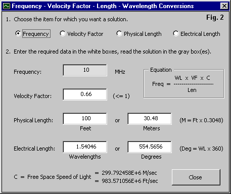
What you input is only a part of what the screen shows, with the rest calculated by the program. You may select one of the common lines available commercially from a long list of options. The list of lines includes the characteristic impedance (Zo), the line velocity factor (VF) and the loss figures, given in TLD as K1 and K2 values. You will enter the length of the line in either a common unit of measure (for example, feet or meters) or in wavelengths. Of course, you will also enter the frequency of concern, since transmission line losses and transformations vary with frequency. If you need to make some conversions either before or after the program does its work, you may go to the conversion screen, shown in Fig. 2. You will also enter the load impedance in series resistance and reactance values. You may set the power input (at the shack end of the line). The program does the rest.
The upper part of the screen toward the right shows the matched loss of the line shown--for RG-8X and 30 MHz, 5.398 dB/100 m. The losses of the 5-m line we are using are 1/20 of that value.
Perhaps the greatest amount of information appears in the lower part of the main screen. The program attempts to place as much information on a single screen as possible. At the lower left, we have tables of values for both the source and load ends of the line. Both columns appear, not only to give us SWR values, but as well because we had a choice when setting in the impedance values earlier: they can be the antenna feedpoint values or the set of values measured at the shack-end of the line.
Note the 2 SWR entries. The upper entry is relative to the Zo of the line, listed at the bottom of the table. The second SWR value is relative to a resistive impedance that we set into the box below the Smith Chart graph in the lower center region of the screen. To the right of the Smith chart, we find a pair of loss columns, one calculated in terms of dB and the other based on the power that we set into the box in the upper screen half. TLD calculates separate values for the losses due to the finite conductivity (mostly of the center conductor of a coax cable but of both conductors of a parallel line) and due to the finite resistivity of the cable dielectric that separates the conductors. In addition, if the line has more than zero-length and we do not have an exact match between the load and the line, there will be added losses due to the effects of SWR, that is, due to the peak voltage and current values that appear along the line. To save you from calculating the percentage of loss due to each factor, the lower right corner of the TLD screen contains a bar graph calibrated to yield the percentage of loss due to each factor.
We can change any of the input values according to the needs of our investigation. For example, we can compare the losses for a specific length of line using RG-8, RG-58, RG-8X, RG-213, and some of the commercial low-loss lines, all by a simple change in the line selection. Even though these are all nominally 50-Ohm lines, we can track the differences in actual characteristic impedance values as we change lines. Many other exercises are equally easy to implement. In addition to coaxial cables, the list of options includes some typical parallel lines.
If we wish to survey the conditions along a length of line, we might wish to try TLW (Transmission Line Program for Windows). The program comes with the current edition (20th as I write) of the ARRL Antenna Book on the enclosed CDROM. Fig. 3 shows the main screen for TLW.

The data that we need to supply is essentially the same as for TLD: line selection; length in meters, feet, or wavelengths; frequency; and impedance as series resistance and reactance values. Note that we can specify the impedance for calculation as either the impedance at the load end of the line or at a given measuring point. Since this screen calculates only in dB, we do not need to specify a power level, although we shall later do so when we explore the "tuner" calculations available to us.
The program revises the line characteristics and the other calculations as we revise any of the input entries. And now we may compare the results between TLD and TLW. For the screen grabs, I supplied both programs with load values of 300 + j100 Ohms and selected RG-8X, using the Belden version of the line. Both line lengths are 5 meters at 30 MHz. However, TLD gives us a shack-end impedance of 23.28 - j61.63 Ohms, while TLW shows 19.36 - j51.65 Ohms. As well, TLD shows a total line loss of 0.742 dB, while the corresponding figure in TLW is 0.854 dB.
Where do the differences come from? What do they mean?
There are differences in the way each program arrives at its final values. However, those difference, whan applied to half wavelength perfect lines, result in differences that are under 0.2%. The major differences occur with respect to the input data cataloged by the program. Note first the difference in velocity factor between the two programs. That small 0.02 difference results in TLW showing a much closer coincidence to TLD values (or vice versa) when the TLW line length increases to 5.1 m. There are also differences in the calculation of matched line losses between the two programs: 5.398 dB/100m vs. 6.320 dB/100 m. There is even a small difference in the listed Zo of the Belden RG-8X: 50.0 - j 0.405 Ohms vs. 50.1 - j 0.47 Ohms. Hence, even using identical calculation procedures, the results would differ.
The important question for the user is whether these difference make a difference? The answer in most cases is "No." Cable specifications represent optimal values given by the manufacturer, and may differ from one batch of cable to the next over a small range. If we change the maker, then the range of difference may be considerably larger. I have measured the VF a non-Belden RG-8X cable as 0.72, which is far from the value used in either program. Perhaps the most divergent figure for the RG-8X cable used in the example is the matched-line loss value.
The upshot of these considerations is that the seeming exact values calculated by the programs are subject to real-world variables, mostly of cable manufacture. (Further deviation between calculations and measurements may also occur due to cable age and conditions of storage, which are user responsibilities.) Calculations within either TLD or TLW are highly useful for study, planning, and designing, but in the end must give way to measurements and adjustments based on those measurements.

For study and planning, TLW has two graphing features that are highly useful. Fig. 4 shows the voltage and current graph that allows you to determine where along the line the peak values occur. Note that I set the power at 1000 watts for both programs for the exercise. The peak voltage with the given load is about 527 Vrms, while the peak current is 10.5 Arms. The peak current on the RG-8X relatively thin center conductor is, of course, a matter of concern, and a more robust cable would normally be used at the frequency and power level of the exercise.

Fig. 5 shows the alternative graph that plots the resistance and reactance along the 5-meter length of transmission line. As in the voltage/current graph, the load end of the cable is at the right, with the transmitter (or tuner) on the left. The line is about 5/8 wavelength. For each half wavelength of the line, notice the length of line over which the resistive component takes on a very low value. As well, notice the reduction in the peak values of both resistance and inductive reactance closer to the source end of the line compared to the comparable values at the load end of the line.

TLW also permits the user to specify a line, such as the one shown in Fig. 6. The screen calls for a relatively complete set of specifications, even for the perfect 450-Ohm line shown here. Proper specification of a line requires not just a resistive impedance, but as well, a reactive component, if there is one. It also calls for a frequency of operation and the attenuation per unit of line, here 100 m. Of course, a velocity factor is mandatory, since even ladder line with only periodic spacers shows a value less than 1.0. As well, every line has a maximum voltage rating that depends on many factors.
The line shown on the sample screen is a perfect 450-Ohm line, that is, a line with no reactance in its Zo, no losses, and a velocity factor of 1.0. Interestingly, when such a line is plugged into TLD at 30 MHz, a load of 2000 - j 2000 Ohms returns the same values at a distance of 1/2 wavelength. In TLW, the calculation process returns 1994.87 - j 1999.86 Ohms for the same initial conditions. The difference is too small to make a difference and is noted simply to show the difference in the calculation procedures for the two programs.
These notes have not covered all of the program features. For example, both programs either show or give an option to show the reflection coefficient as an alternative to the SWR value that amateurs so commonly use. TLD has loss values applicable to the Sonata suite of engineering modeling programs, and it provides a graph of matched line losses for a wide range of frequencies. TLW has calibrated results based on noise-bridge or Autek antenna analyzer measurements. The unique features of each program justify having both available for ready use, especially since they come at essentially no cost (or, in the case of TLW, at no extra cost).
Clemens Paul, DL4RAJ, has reminded me that there is a free on-line program (Transcalc) by Kevin Schmidt, W9CF, at his website: w9cf.github.io . Although the program notes that it uses a number of features from TLW, the calculation procedure appears to resemble more the one used by TLD in terms of results from specifying lossless or perfect lines. TLD does not calculate SWR's above 999, but Transcalc does. Additionally Transcalc shows graphically what is happening along the line like TLW, and also has a zooming feature. The W9CF applet contains instructions for downloading two files that together allow storage of the program locally for use with your browser in the off-line mode. For offline use of Transcalc with newer Windows versions (such as XP), you have to download the (free) MS virtual machine or the java plug-in from Sun. For basic transmission-line calculations and a graph of voltage, current, and power along a long length of line, the W9CF program can be very useful as an alternative to the ones reviewed in these notes.
Tuner Analysis
The analysis of antenna tuners is at root the analysis of networks effecting an impedance match between a user-specified load impedance and either a given or user-specified source impedance. Most usually, the source impedance (Rin) is 50-Ohm resistive. However, the load impedance may be complex.
Programs vary in how many networks they include. For example, TLW includes the most common networks used in tuners used by radio amateurs: the low- and high-pass L, the low-pass (CLC) PI, and the high-pass (CLC) T. A suite of utility programs by Brian Eagn, ZL1LE, adds the low-pass (LCL) T as well as a collection of 2-element networks. A more general program called the "Impedance Matcher" includes a total of 16 networks, including a number of "double Ls" (which may go under different names in other contexts, such as the PI-L sometimes used in power amplifier design).
We shall examine briefly the 3 programs noted, but not because they vary in the number of networks offered. Rather, each program begins its calculations at a different point, and these differences are notable in terms of the responsibility they place on the user.
Network analysis begins with two sets of numbers besides the impedances to be matched. For convenience, the sample load (Zout) will always be 300 + j 100 Ohms, and the input impedance (Rin) will be 50 Ohms. One additional set of figures is the unloaded or component Q (or Qu) of the capacitor(s) and inductor(s) in the network. For the purposes of this survey, inductor Qu will be 250, and capacitor Qu will be 5000. Each of those values will vary according to the component quality and to the circumstances of use. With a roller inductor or a tapped coil, the Q may vary widely over the frequency range as the ratio of coil length to coil diameter changes, and the contribution to inductance of the leads rises with frequency. The component Q-values that I have chosen are generous.
The other figure of importance is delta (as defined in Terman). Where available, the Greek letter uses the lower case. To avoid finding a lower case delta on a keyboard, the term now has a variety of names, all using the letter Q: effective Q, loaded Q, network Q, and operating Q, to name a few. Vacuum-tube amplifier output PI networks tend to use delta values around 10-12, while solid-state amplifiers aim for values closer to 1. The value of delta makes a difference to tuner losses. In general, power lost/power delivered to the load is equal to delta/Qu (where for first order approximations, one might use the Qu of the inductor). Therefore, network efficiency as a percentage equals 100 * (1 - delta/Qu). Therefore, the higher the component Q and the lower the delta, the more efficiently the tuner will transfer power from the source to the load. (The load, of course, is usually a system that includes an antenna plus a transmission line, and the line--as we have seen--may have losses of its own.)
One factor not included in network calculations is the fact that for very low values of delta, the settings of components for a perfect match to a 50-Ohm source and the settings for maximum power transfer may differ slightly. When delta is greater than about 10, the differential is virtually undetectable. However, when delta drops down to the 1-3 range, those settings may differ by amounts detectable from variable component settings. (See Chapter 6 of recent editions of The ARRL Handbook for more on this phenomenon in parallel tuned circuits.) Because most tuners do not include relative output indicators, most users settle for a perfect impedance match rather than for maximum power transfer. Nevertheless, the most ideal tuner component values are those that yield the lowest value of delta.
TLW includes--besides the transmission-line analysis--a supplementary module for tuner analysis. The module is based on the older DOS program, AAT. In the TLW context, it uses for its impedance input the values calculated for the source end of the transmission line. However, if you wish to directly input a value, just specify any transmission line with a length of zero. Then the load impedance from the main screen will also appear at the load terminals of the network.

Fig. 7 shows the tuner selection screen, with its options. The power setting also applies to the main page. The component Q values are the default values, although for this exercise, we have altered them. As well, the selections provide a value for stray capacitance at the network output, using a default value of 10 pF. In the following exercises, I have reduced this value to zero so that calculations among programs will correlate to the degree possible. However, for practical tuner analysis, the stray capacitance value can be very useful, especially when looking at the performance of a given tuner on the 12- and 10-meter bands, where 10 pF is a large percentage of a network's output capacitance.
The calculations for high-pass (Cs-Lp, where Cs is a series capacitor followed by Lp, a parallel or shunt inductor) and low-pass (Ls-Cp) L networks are quite standard. Fig. 8 shows both screens for a tuner load impedance of 300 + j100 Ohms. If we first calculate the delta (or effective Q, in this program), then there is only one set of component values that will meet that delta calculation and still yield a match to the 50-Ohm input.

TLW, as shown in Fig. 7, allows matching calculations for only 2 other tuner networks in common use: the low-pass (Cp-Ls-Cp) PI and the high-pass (Cs-Lp-Cs) T. Fig. 9 shows the calculations for both of these networks for the specified conditions. It also shows the approach taken to solving the requisite equations for these networks.

Note that each network has an output-side capacitor whose value is an integer. For each network, the user must select the value of that component, and the program completes the calculations, including deriving the delta or effective Q of the network. If the goal is the most efficient transfer of power, then the user must try different values for the output-side component until the effective Q value reaches its lowest value. The required value may not be the highest or lowest value for which there is a solution to the network equations. For example, output capacitance values between 35 and 45 pF all calculated a delta of 1.6 for the high-pass T network. However, there may be values for which there are no solutions, and the program prompts you for a different value.
A program that takes quite a different approach to the calculations is known as Impedance Matcher (or more correctly, as Impedance Matching Network Designer). This program is a scripted on-line calculator, but you may download the entire file, with its subdirectory of graphics, and run the program locally on your browser. The URL is bwrc.eecs.berkeley.edu/Research/RF/projects/60GHz/matching/ImpMatch.html (web.archive.org). The script covers 16 networks, of which Fig. 10 shows the most common ones used in amateur antenna tuners.

The page shows only solutions for the low-pass and high-pass L networks. The reason for this condition is the required input data. Besides the input and output impedances and the frequency (in basic units), the user must supply a target value for delta called the Desired Q in this treatment. The value prescribed is 2.0. The L network calculations provide the values for the closest value of desired Q, but the other networks make use of the specified Q. Hence, they have no solutions. There are solutions for a delta of 2.4, and we shall shortly look at them in comparison with the values produced by the other programs.

Fig. 11 shows the remainder of the single long page of possible networks in the program. For a desired Q of 2.0, there are some solutions among the "LL" circuits, although we normally do not find these in antenna tuners. However, all of the more complex matching networks have places in solid-state amplifier designs and in numerous other applications.
So far, we have looked at two approaches to network calculations. For networks having 3 components, TLW has the user specify the output-side component value and search for the lowest delta. Impedance Matcher has the user select a desired Q and then adjust that value until the program provides a solution in terms of component values. There is a third route to network solutions, the one used in one of the GW Basic HamCalc suite of utilities. You can find the latest version of Hamcalc at www.cq-amateur-radio.com/HamCalcem.html (web.archive.org). In the index, find the program called Transmatch Design by Brian Egan, ZL1LE. Because Basic screens do not register as graphics on my operating system, we shall have to content ourselves with text-grabs from those screens.
The calculations for L networks (called Ladder networks in the program) generally do not stray far from the techniques used in the other programs. The following example of a low-pass L (Cs-Lp) makes that clear. We begin by entering the required input data, and the program specifies which type of network will provide a solution. Note that the components are specified simply as reactance positions. The program will not only provide solutions involving the usual cases in which we have a series reactance of one type and a shunt reactance of the other type. There are conditions of load impedance that may require series and parallel reactances of the same type. However, we shall not encounter them with our simple 300 + j100 Ohm load transformed to 50 Ohms resistive. The text-grabs will not reproduce the special characters used to show some of the network diagrams (created by HamCalc's master, George Murphy, VE3ERP). Still, you likely can infer what goes where. R1 always refers to the input impedance and R2 and X2 refer to the output or antenna-side impedance.
                   2-ELEMENT LADDER MATCHING NETWORK PROGRAM
---------------------------- by Brian Egan, ZL1LE ------------------------------
    TYPE 'A' LADDER NETWORK               TYPE 'B' LADDER NETWORK

      o--- Xa ---------o                    o--------- Xa ---o
                 |                                |
      ---»       Xb   ---»                  ---»  Xb       ---»
      R1         |   Load                   R1    |        Load
       ----------------                      ----------------
-------------------------------------------------------------------------------
                   +------------------------------+
                   |  NETWORK DESIGN PARAMETERS:  |
                   +------------------------------+

1.   ENTER frequency of operation in MHz:   30
2.   ENTER value of input resistance, R1, in ohms:  50
3.   ENTER value of load resistance, R2, in ohms:   300
4.   ENTER value of load reactance, X2, in ohms:    100

-------------------------------------------------------------------------------
a TYPE A network is required to match prescribed source and load.
-------------------------------------------------------------------------------
The network requires a Type A network, but it has two forms, as shown by the following grabs of the solutions.
                   2-ELEMENT LADDER MATCHING NETWORK SOLUTIONS
-------------------------------------------------------------------------------
+------------------------------------------------------------------------+
| DESIGN PARAMETERS:                           LOAD SWR  =   6.68        |
+------------------------------------------------------------------------|
| Frequency (MHz)    =    30           Load Resistance  =  300.0 _       |
| Source Resistance  =    50.0 _       Load Reactance   =  100.0 _       |
+------------------------------------------------------------------------+
-------------------------------------------------------------------------------
    SOLUTION 1.              o--- Ca ---------o
    ----------                          |
Ca (pF) =   44.6             ---»       Lb   ---»
Lb (uH) =  0.864             R1         |   Load
delta   =  2.05               ----------------
-------------------------------------------------------------------------------
    SOLUTION 2.              o--- La ---------o
    ----------                          |
La (uH) =  0.631             ---»       Cb   ---»
Cb (pF) =   43.2             R1         |   Load
delta   =  2.38               ----------------
-------------------------------------------------------------------------------
The differences between the ZL1LE approach and the others that we have encountered show up once we work with 3-component networks. Let's begin with the low-pass PI (Cp-Ls-Cp). In the text-grab below, the component graphics do not show correctly. As well underlines appear instead of the omega for Ohms and the delta for the effective or network Q.
                         PI-COUPLER TRANSMATCH DESIGN
--------------------------------------------------------------------------------
                                       L
                          R1 »-------_____-------» RL
                          input  |           |   load
                                -+- C1      -+- C2
                                 |           |
                           grnd ///         ///
--------------------------------------------------------------------------------
        Transmatch Input Impedance R1................   50.00 _
        Load Resistance RL...........................  300.00 _
        Load Reactance...............................  100.00 _
        Frequency....................................   30.000 MHz
        Inductor L...................................    0.684 uH
        SWR..........................................    1:1
 SOLUTION 1:  ( _[delta] = 2.9 )
        Capacitor C1.................................   35.72 pF
        Capacitor C2.................................   45.64 pF
 SOLUTION 2:  ( _[delta] = 3.1 )
        Capacitor C1.................................   46.57 pF
        Capacitor C2.................................   47.27 pF
--------------------------------------------------------------------------------
Note that the inductor value appears above the section of the screen devoted to solutions. The reason for the placement is that the program first calculates the maximum value of inductor, in this case 0.685 uH. Due to rounding, the program may not always accept this value as the user input, and so, as shown above, you must select a notch lower than maximum. The procedure has two goals. First, it allows direct calculation to the lowest feasible value of delta--2.9 in this case. However, that goal must also coincide with the derivation of multiple solutions, if they exist. Hence, in some case, you may be able to adjust the value of the networks required component input value and arrive at one of the two solutions with a marginally lower value for delta.
Transmatch Design also provides calculations for the low-pass T (Ls-Cp-Ls), an underused but effective tuner network. In this case, the program pre-calculates the minimum value for the input-side inductor. In the following text-grab, you will find that I had to replace the minimum 0.631 uH value with 0.632 uH.
                         LOWPASS TEE TRANSMATCH DESIGN
--------------------------------------------------------------------------------
                                  L1       L2
                          R1 »---____-----____---» RL
                          input        |         load
                                      -+- C
                                       |
                                      /// grnd
--------------------------------------------------------------------------------
        Transmatch Input Impedance R1................   50.00 _
        Load Resistance RL...........................  300.00 _
        Load Reactance...............................  100.00 _
        Frequency....................................   30.000 MHz
        Inductor L1..................................    0.632 uH
        SWR..........................................    1:1
 SOLUTION 1:  _[delta]=  2.4
        Capacitor C..................................   43.20 pF
        Inductor L2..................................    0.00 uH
 SOLUTION 2:
        No second solution
--------------------------------------------------------------------------------
For this network, there is only one solution, and the value of delta is quite in line with values that we have seen for other networks. Hence, despite the erroneous impression that "too many" inductors will ruin tuner efficiency, the value of delta tells a different story. However, note that for the matching condition specified, the output inductor goes to zero. The result is an L-C-L T that is effectively a low-pass L network.
In his original formulation of the high-pass T (Cs-Lp-Cs) network calculations, ZL1LE used equations comparable to those used for the other 2-component networks. However, he revised his calculations following the QEX article "Estimating T-Network Losses at 80 and 160 Meters" by Kevin Schmidt, W9CF (July, 1996). [This article is often mis-referenced as appearing in July, 1997.] For further notes on this network, see "Understanding the T-tuner (C-L-C) Transmatch" by William E. Sabin, W0IYH, QEX (December, 1997).
ZL1LE's re-formulation of the high-pass T calculations now yield a table of values based on the inductor Q values.
 HIGH-PASS TEE TRANSMATCH (with finite Q inductor)
--------------------------------------------------------------------------------

                        Input >---|+---------|+---> Load
                                  C1    |    C2
                                  +_____+
                                  |  L
                                \\-\\

--------------------------------------------------------------------------------
 ENTER: Input impedance in ohms......? 50
 ENTER: Load resistance in ohms......? 300
 ENTER: Load reactance in ohms.......? 100
 ENTER: Frequency in MHz.............? 30
--------------------------------------------------------------------------------

 HIGH-PASS TEE TRANSMATCH (with finite Q inductor)
--------------------------------------------------------------------------------
 DESIGN PARAMETERS:| R1=  50.0 _| RL= 300.0 _| XL= 100.0 _| Freq.=  30.000 MHz
--------------------------------------------------------------------------------
                      TABULATION OF TRANSMATCH PARAMETERS
         +-----------------------------------------------------------+
         |    Q    |  L(uH)  |  C1(pF) |  C2(pF) |Loss (dB)| Eff.(%) |
         +---------+---------+---------+---------+---------+---------|
         |Infinite |  0.699  |   47.4  |   47.1  |  0.00   |  100.0  |
         |   250   |  0.680  |   47.4  |   40.2  |  0.04   |   99.0  |
         |   200   |  0.677  |   47.4  |   39.2  |  0.05   |   98.8  |
         |   150   |  0.673  |   47.4  |   37.8  |  0.07   |   98.4  |
         |   100   |  0.665  |   47.4  |   35.6  |  0.11   |   97.6  |
         |   50    |  0.649  |   47.4  |   31.3  |  0.22   |   95.0  |
         +-----------------------------------------------------------+
--------------------------------------------------------------------------------
Using the values for an inductor Q of 250, we can back calculate the value of delta at 2.4. The ZL1LE calculation procedure aims directly at the lowest feasible value of delta to produce component values capable of maximum power transfer. In tuners--but not in all applications of networks--this is the user's goal in setting variable components.
We should pause to examine a significant question apart from the procedures necessary within each program to yield component values for the lowest feasible value of delta. The question is simply a matter of whose calculation to believe. To point toward an answer--without necessarily arriving at a final decision--let's catalog the values for networks where at least 2 of the programs produce solutions. We can work through the networks in order, remembering that in each case, the design frequency is 30 MHz, the source impedance is 50 Ohms resistive, and the load impedance is 300 + j100 Ohms. The inductor Qu is 250 and the capacitor Qu is 5000, wherever those figure may play a role in the calculations. You may calculate the efficiency and the loss from the equations with which we began these tuner network notes.
1.  High-Pass (Cs-Lp) L Network
Parameter         TLW             Imp. Matcher        Trans. Design
Cs (pF)           44.8            44.6                44.6
Lp (uH)           0.86            0.863               0.864
delta             2.4             2.38                2.05
The only difference among the 3 is the Transmatch Design calculation of the delta value. However, the difference results only in a 0.2% change in efficiency, an amount that would not be detectable by ordinary means of measurement.
2.  Low-Pass (Ls-Cp) L Network
Parameter         TLW             Imp. Matcher        Trans. Design
Ls (uH)           0.63            0.631               0.631
Cp (pF)           43.4            43.2                43.2
delta             2.4             2.38                2.38
So far, we have nothing to choose relative to the 3 programs. Perhaps there will be some significant differences among the 3-component networks.
3.  Low-Pass (Cp-Ls-Cp) PI Network
Parameter         TLW             Imp. Matcher        Trans. Design
Cp (pF)           17.2            37.8                35.7     46.6
Ls (uH)           0.66            0.684               0.684    0.684
Cp (pF)           44.0            45.9                45.64    47.27
delta             2.7             2.40                2.90     3.10
The Transmatch Design double solution values bracket those produced by Impedance matcher. Although the TLW values appear on the surface to be more distant, note the 11 pF spread between the two Transmatch Design solutions. The TLW input capacitor value is not so far out of range as it may seem, when we consider that for low values of delta, tuning is often very broad. Had I chosen a different output capacitor value, the input capacitor value would have come into closer alignment without unnecessarily disturbing the value of delta. Again, a few tenths difference in delta will make no significant difference to the tuner's efficiency.
4.  Low-Pass (Ls-Cp-Ls) T Network
Parameter         TLW             Imp. Matcher        Trans. Design
Ls (Ls)           ----            0.636               0.632
Cp (pF)           ----            43.3                43.2
Ls (uH)           ----            0.036               0.0
delta             ----            2.40                2.40
Once more, there is no significant difference between the two programs that provide results for the low-pass T network.
5.  High-Pass (Cs-Lp-Cs) T Network
Parameter         TLW             Imp. Matcher        Trans. Design
Cs (pF)           47.6            44.2                47.4
Lp (uH)           0.69            0.651               0.680
Cs (pF)           45.0            ----                40.2
delta             1.6             2.40                2.40
The anomalous solution to the C-L-C T appears in the Impedance Matcher program. In the output capacitor value box, it lists "NaN," indicating that there is no calculable value. Varying the desired Q over a wide range makes no difference to that solution box. In contrast, the values produced by TLW and Transmatch Design are closely coincident, despite the difference in the calculated value of delta. (After I wrote this item, TLW incorporated revisions that should eliminate differences in the calculation of delta.)
In the end, there is little to differentiate the final calculations among the 3 styles of network calculation programs. The main differences lie in the approach to the calculations. For network calculations that aim directly at the lowest feasible value of delta, perhaps Transmatch Design is the most straightforward. However, its GW Basic format is far less convenient than the Windows format used by TLW.
In addition, TLW provides extensive information about probable component losses as well as the total tuner loss. It also supplies the peak voltages across capacitors and the RMS current through inductors--for the power setting chosen--as a guide for safe design or use of the tuner. Consequently, as a package, TLW may be the most complete tuner analysis program around, even if the user must fish a bit to arrive at the lowest effective Q or delta.
Since the three programs are no cost items (or for TLW, a no-cost extra), you can afford to have all of them available in order to use each where it may be strongest. As well, both TLD and TLW provide complementary coverages of transmission-line analyses at no cost to the user. In essence, then, we have a suite of calculation programs that can go a long way toward giving us a complete picture of what is occurring electrically between the antenna feedpoint and the transceiver input/output. What the birds and weather may be doing to the system is another matter entirely.
Updated 01-01-2005. © L. B. Cebik, W4RNL. This item first appear in antenneX for December, 2004. Data may be used for personal purposes, but may not be reproduced for publication in print or any other medium without permission of the author.