There is an urge among antenna builders to discover "magic formulas" for determining the element lengths of various antenna types. In most cases, tradition sets the form of these formulas in the following terms:

We seek the length in customary dimensional units (and "dim" may equal feet, inches, meters or millimeters) using some constant, K, and the frequency, f, in MHz.
Except for the simplest of antennas, we should wean ourselves from this urge. Antenna dimensions do not tend to scale in such simplistic terms. Even the simple 1/2 wl dipole resonant length varies with wire size and height above ground. Hence, using a cutting formula becomes a matter more of luck than of antenna knowledge.
More complex antennas tend to be less prone to performance variations created by antenna height, if the antenna is at least 1/2 wl high. The more closed the structure of the antenna, the more immune it becomes to variations in resonant element length by virtue of height above ground. However, nearly all common types of antennas will vary according to the diameter of the element size.
In most cases, dimensional differences will be negligible between antennas built of materials with perfect conductivity and those using ordinary materials such as copper and aluminum. A difference is negligible if it falls within the margins of error that are inherent in standard construction practices. For home shop construction practices, a 1 to 2 percent dimensional error range is normal. Of course, the more elaborate the shop and the more experienced the builder, the smaller the potential error range.
In the end, then, we are left with the diameter of the element wire (or rod or tubing) as the key to determining the element length. One common warning that we give with respect to scaling antennas for other than the design frequency is also to scale the wire diameter. Only under this condition will the scaling play true. In addition, we must also attend to element length differences between uniform-diameter elements and those which are tapered in steps, normally from a large diameter at the element center to a small diameter at the tip. Likewise, different tapering schedules may result in different element lengths for the same frequency and materials.
A Procedure for Developing Sensible Design Equations
If we work initially with uniform-diameter elements, it is possible to develop design equations for many antenna types. The starting point will normally be the element diameter. Again, the equations should begin using perfectly conductive material, with any necessary adjustments for real materials made later. The question then becomes how we may develop such equations. To answer the question, we may turn to an example.
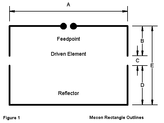
Fig. 1 is the outline of a Moxon Rectangle, a two element array that combines mutual coupling between elements and coupling between the element tips to yield a broad forward lobe with nearly the strength of a 2-element driver-reflector Yagi. The pattern is almost cardioidal so that minimum radiation does not occur 90 degrees off the main lobe, but closer to 120 degrees away. The antenna at its design frequency is capable of better than 30 dB front-to-back ratio, with better than 20 dB front-to-back ratio across most HF amateur bands. Because the side-to-side dimension of the antenna is only about 70% of the width of a full-size 2-element Yagi, the antenna has found interest among those with limited space. Further interest has arisen among those who can put the antenna pattern to good use. An additional advantage of the design is the 50-Ohm feedpoint impedance, which simplifies matching requirements. A considerable bibliography on the antenna is available from British, American, and Australian sources, as well as at my web-site (..).
Our interest in the antenna stems from the designations of the element dimensions, listed as A through E in Fig. 1. By judicious modeling in NEC (version 2, 3, or 4), one can develop fairly precise models to create a base-line data set for the development of some design equations. However, the data set must meet standards for use as the basis for this development. For the Moxon Rectangle, I set these standards for each model in the data set.
Free-Space Gain Range:              5.95-6.05 dBi
180-Degree Front-to-Back Ratio:     >35 dB
Source Impedance: Resistance:       50-54 Ohms
                  Reactance:        <+/-1 ohm
The next step is to decide upon the wire diameters to use for development purposes. Several factors enter into this decision.
Common antenna building materials include AWG wire sizes (in the U.S.) and aluminum tubing and rods ranging from 1/8" to over 1" in diameter. For reference, the following table lists commonly used AWG wires sizes and their diameters in various units of measure.
AWG Size          Dia. Inches             Dia. Feet               Dia. mm
18                .0403                   0.003358                1.0236
16                .0508                   0.004233                1.2903
14                .0641                   0.005342                1.6281
12                .0808                   0.006733                2.0523
10                .1019                   0.008492                2.5883
As useful as these conversions may be, they will not satisfy the needs of developing design equations. The wire size used must be given in terms of a fraction of a wavelength, and this number will vary with frequency for any given physical wire size. To provide a sense of the range of wire sizes, when given in terms of wavelengths, the following table presents some materials that have been used in published antenna projects, with the element diameter given in wavelengths for various frequencies.
      Wire                                Frequency (MHz)
Size        Dia.(")           1.8         7           28          50          144
AWG #18     0.0403            6.146E-6    2.390E-5    9.560E-5    1.707E-4    4.917E-4
AWG #14     0.0641            9.775E-6    3.802E-5    1.521E-4    2.715E-4    7.820E-4
AWG #10     0.1019            1.554E-5    6.043E-5    2.417E-4    4.317E-4    1.243E-3
1/4"        0.25              3.813E-5    1.483E-4    5.931E-4    1.159E-3    3.050E-3
1/2"        0.50              7.625E-5    2.965E-4    1.186E-3    2.118E-3    6.100E-3
1"          1.00              1.523E-4    5.931E-4    2.372E-3    4.236E-3    1.220E-2
In practical terms, the range of wire sizes--given in terms of a fraction of a wavelength- -runs between about 1E-5 and 1E-2. Extending the range to thinner wires presents no problems, although it is not especially useful. However, at the upper limit, there is a potential modeling problem. The Moxon "tails" (dimensions B and D in Fig. 1) require proportional segmentation to the parallel wires (dimension A). For good convergence, I chose to set B at 5 segments and D at 7 segments, with A using 35 segments. As the wire diameter approaches 0.01 wl, the wire diameter begins to exceed the segment length. Ideally, the segment length should be considerably greater than the wire diameter. Hence, the modeled results become less reliable with the fattest wires in the set. (A model with only linear elements would not present this difficulty, and a lower level of segmentation might well be used with excellent reliability.)
The next step is to decide what wire-size steps to use in developing the base-line data set. In most cases, antenna dimensions tend to show changes that relate to the logarithm of the wire size rather than to linear steps in wire size. For the range of wire sizes shown, we can conveniently take the common log of wires sizes from 1E-5 through 1E-2 to get a progression of logarithms from -5 to -2 in integral steps. However, the data set would be very small. To keep the log steps linear, we may take intermediate wire sizes from 3.162E-5 through 3.162E-3 to obtain values for the common logs -4.5 through -2.5. How much finer one might wish to go depends very much on the rate of variation of values and the anticipated complexity of the resultant curves. For this project, the seven data sets provided a sufficiently large basis for the development of design equations.
The following table lists the results of the modeling exercise, showing the free-space gain, 180-degree front-to-back ratio, feedpoint impedance, and dimensions A-E (in wavelengths) for the models.
1.  Performance Parameters
Wire Size   Log         Gain        Front-to-Back     Feedpoint Z
(wl)        (base 10)   (dBi)       Ratio (dB)        (R+/-jX Ohms)
1E-5        -5          6.04        48.1              52.5 + j 0.4
3.162E-5    -4.5        6.06        39.2              51.5 + j 1.0
1E-4        -4          6.03        41.8              52.5 - j 0.8
3.162E-4    -3.5        6.01        36.1              52.5 + j 0.6
1E-3        -3          6.00        41.7              53.0 - j 0.7
3.162E-3    -2.5        5.95        35.4              53.3 - j 0.8
1E-2        -2          5.95        35.0              53.9 + j 0.8

2.  Dimensions (See Fig. 1)
Wire Size               Dimensions in Wavelengths
                  A           B           C           D           E
1E-5              0.366       0.057       0.007       0.067       0.131
3.162E-5          0.366       0.056       0.009       0.067       0.132
1E-4              0.364       0.055       0.010       0.068       0.133
3.162E-4          0.364       0.053       0.012       0.068       0.133
1E-3              0.360       0.051       0.013       0.069       0.133
3.162E-3          0.358       0.046       0.018       0.069       0.133
1E-2              0.356       0.040       0.024       0.070       0.134
The front-to-back ratios of the base-line models seem to vary considerably. However, the peak 180-degree front-to-back ratio--which may reach 50 dB in models--is a very narrow band phenomenon. Hence, values between 35 dB and 45 dB may be only a few kHz apart.
In order to maintain a feedpoint impedance close to 50 Ohms, the side-to-side dimension (A) must decrease as the wire size increases. One expected result would be an increase in the driver tail length (B). However, the increasing wire diameter overrides this increase and results in a shortening of the tails as well as the side-to-side dimension. The reflector is less affected by the changes in wire diameter and shows an increase in tail length (D) with the shortening of A.
Most evident and rapid is the increase in dimension C, the gap between the tips of the driver and reflector tails. As the wire size increases, the degree of coupling between tips also increases. To sustain roughly equivalent performance across the base-line set of models, the gap must be increased in an ascending curve. The greatest increases in the table do occur where the models begin to show reduced reliability. However, the general trend holds true. Note that the overall front-to-back dimension (E) does not change much over the entire range of wire sizes.
Step-wise (rather than smooth) variations occur in the tabulated results because the increments of dimensional change were limited to 0.001 wl. For almost identical performance, there is a small range of values for the gap. (If there were not, the antenna would be difficult to reproduce.) Centering the gap value within its range would have yielded smoother curves for all of the dimensions. However, this degree of precision would have been superfluous to the effort.
From Data to Equations
The data set generated by the base-line models is sufficient to develop design equations. The easiest way to develop usable equations is to subject the data to regression analysis, which is available in many mathematical software packages, either in stand-alone form (such as DataFit) or in larger suites of functions. Although a significant description of regression techniques is well beyond the scope of these notes, we can indicate the process and its output.
For any data set--especially where the plotted data has a linear X axis scale--regression analysis can develop polynomial equations that best fit the data. The routines can produce any order of polynomial. For example, the form most used in the following discussion is a 2nd order polynomial of the form
where a, b, and c are coefficients generated by the regression analysis, (for our case) x is the common log of the wire diameter, and y is the dimension under analysis. Dimensions A, B, and C require second-order polynomials, while dimension D can be satisfied with a first order equation.
In any such exercise in regression analysis, it is important to understand that the equations developed have no inherent physical meaning relative to antenna theory or practice. The results are simple curve-fitting exercises within the upper and lower limits of the values for X and the data supplied. However, the results are usable in practice with some care. Foremost is the need to determine when a generated equation is adequate to a given task. Although in complex cases, the test routines report important information by which to evaluate the equations, simply plotting the equations against the data points can--in simpler cases--provide enough information to decide which level of polynomial will satisfy the needs of a project. For the present data set, one significant factor is that the equations should not result in extreme departures from the modeled data at the limits of the values for x. For A through C, 2nd-order equations sufficed, and for D, a first order equation (ax + b) proved sufficient. (In other cases, I have used up to 4th-order polynomials.)
To establish the fits, the following graphs of dimensions A though D may be useful.
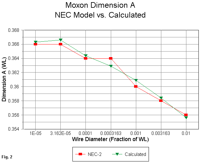
Fig. 2 shows a comparison of modeled and calculated values for dimension A. Within any normal building tolerances, this curve is a very tight fit.
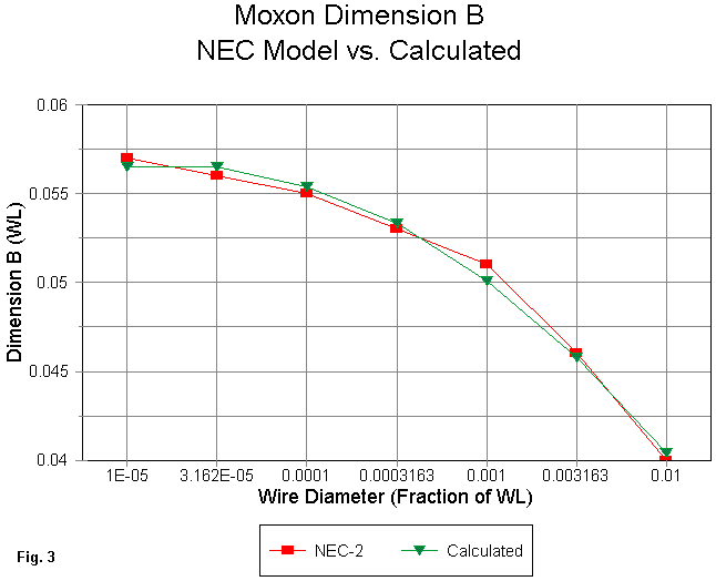
A comparison of modeled and calculated values for dimension B (the driver tail) appears in Fig. 3. This curve is an even tighter fit than for dimension A.
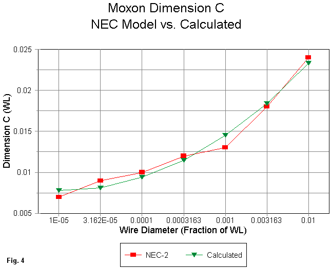
Fig. 4 shows a comparison of modeled and calculated values for dimension C, the gap between element tips. The modeled values do not have enough significant digits for a smooth curve.
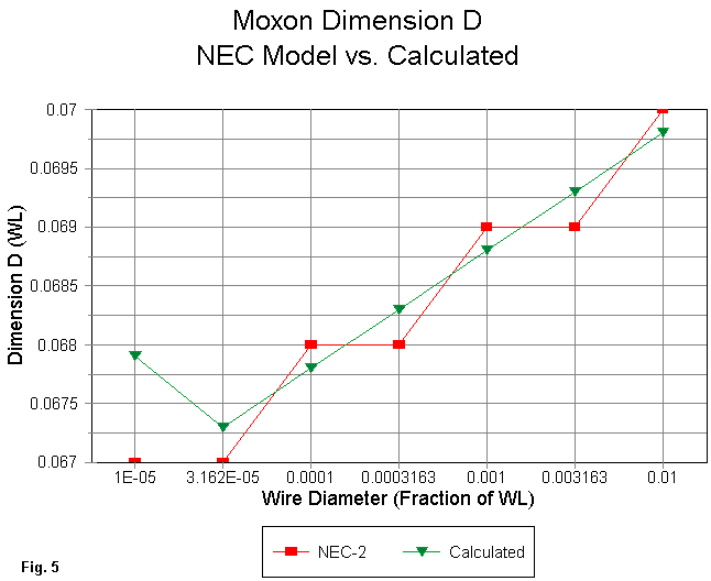
A comparison of modeled and calculated values for dimension D (the reflector tail) appears in Fig. 5. The sharpness of turns in both curves is due to the very small change overall on dimension D.
I have not yet shown the values for the coefficients, because they will appear shortly within each of the two methods I have selected for packaging the results. However, it should be apparent that all of the curves fit the data reasonably well, given the increment of change within which the models were developed. It cannot be stressed enough that a. the equations have no direct theoretical meaning within antenna theory and b. care must be used to ensure that the equations are neither more complex than they need to be for a task nor too simple to capture the essential data within the limits of the defined range of values.
Packaging the Design Equations
There are innumerable ways to package the design equations in order to make them usable and convenient. We shall look at only two here.
1. A Basic (or other language) utility program: The following listing provides a small utility program for calculating Moxon dimensions from an input of the wire diameter and the design frequency. The wire diameter may be input in inches, millimeters, or wavelengths. The output is given in wavelengths, feet, and inches. The simple addition of a few lines converting the English output into metric units (0.3048 * feet) would complete the program.
10 CLS:PRINT "Program to calculate the dimensions of a Moxon Rectangle."
20 PRINT "All equations correlated to NEC antenna modeling software for wire diameters"
30 PRINT "     from 1E-5 to 1E-2 wavelengths."
40 PRINT "L. B. Cebik, W4RNL"
50 INPUT "Enter Desired Frequency in MHz:";F
60 PRINT "Select Units for Wire Diameter in 1. Inches, 2. Millimeters, 3. Wavelengths"
70 INPUT "Choose 1. or 2. or 3.";U
80 IF U>3 THEN 60
90 INPUT "Enter Wire Diameter in your Selected Units";WD
100 IF U=1 THEN WLI=11802.71/F:DW=WD/WLI
110 IF U=2 THEN WLI=299792.5/F:DW=WD/WLI
120 IF U=3 THEN DW=WD
130 PRINT "Wire Diameter in Wavelengths:";DW
140 D1=.4342945*LOG(DW)
150 IF D1<-6 then 160 else 170
160 print "Wire diameter less than 1E-6 wavelengths:  results uncertain."
170 if d1>-2 THEN 180 ELSE 190
180 PRINT "Wire diameter greater than 1E-2 wavelengths:  results uncertain."
190 AA=-.0008571428571#:AB=-.009571428571#:AC=.3398571429#
200 A=(AA*(D1^2))+(AB*D1)+AC
210 BA=-.002142857143#:BB=-.02035714286#:BC=.008285714286#
220 B=(BA*(D1^2))+(BB*D1)+BC
230 CA=.001809523381#:CB=.01780952381#:CC=.05164285714#
240 C=(CA*(D1^2))+(CB*D1)+CC
241 DA=.001:DB=.07178571429#
242 D=(DA*D1)+DB
243 E=(B+C)+D
250 PRINT "Moxon Dimensions in Wavelengths:"
260 PRINT "A = ";A
270 PRINT "B = ";B
280 PRINT "C = ";C
290 PRINT "D = ";D
295 PRINT "E = ";E
299 WF=983.5592/F:WFI=WF*12:PRINT "Wavelength: =";WF;"Feet or ";WFI;"Inches
300 PRINT "Dimensions in Feet and Inches"
301 PRINT "A = ";A*WF;"Feet or ";A*WFI;"Inches"
302 PRINT "B = ";B*WF;"Feet or ";B*WFI;"Inches"
303 PRINT "C = ";C*WF;"Feet or ";C*WFI;"Inches"
304 PRINT "D = ";D*WF;"Feet or ";D*WFI;"Inches"
305 PRINT "E = ";E*WF;"Feet or ";E*WFI;"Inches"
350 INPUT "Another Value = 1, Stop = 2: ";P
360 IF P=1 THEN 10 ELSE 370
370 END
Lines 190 through 243 contain the design equations and coefficients derived from the regression analysis. The variable names AA through DB should be self-explanatory. Note that the calculations use the log of the wire diameter in wavelengths, and not the wire diameter itself. Dimension E is the simple sum of B, C, and D. It serves as a check on the fittingness of the other calculated dimensions by comparing it with the corresponding modeled value. Additionally, I have expressed the coefficients and other constants to full calculated values, rather than using truncated values based on the least significant digits of any entry. The resulting output values can easily be trimmed by the user at any sensible level.
With the calculated dimensions in hand, one can create a model of the Moxon as a check, as a basis for optimization in models, or as a guide to building. The side-to-side dimension with require halving in order to place the front-to-back axis along the center-line of the antenna in any NEC model.
2. Development of a model by equation: The equations can also be entered directly into a NEC program that has the facility to accept design-by-equation. As an example, Fig. 6 shows the equations screen for a NEC-Win Plus model.
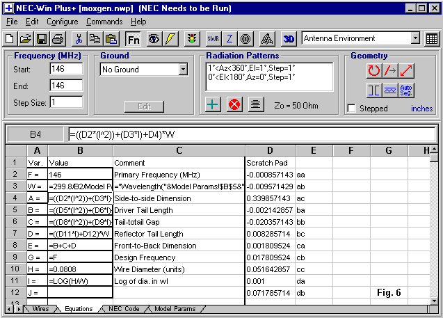
Only one of the equations appears fully in the upper entry line, but it suffices to show the parallel to the Basic program. The spreadsheet does know the difference between natural and common logarithms, so the calculation of the log of the wire diameter in wavelengths (variable I) has a different meaning of "LOG" from its meaning in Basic. (Common GW Basic uses only natural logs and hence requires a conversion factor to yield common logs.)
The list of coefficients is entered in column D. As the sample equation for box B4 indicates, the equations of the dimension variables call upon the locations of the coefficients to employ their values in the calculation. Column E contains the identification of each coefficient, using the same labels as in the Basic listing.
The advantage of entering the equations directly into a modeling program is that one can then design a Moxon for any reasonable frequency with any reasonable wire diameter and evaluate the model--all in one operation. One of the variable entries equates the design frequency with the current frequency. However, you can lock in a set of dimensions by simply entering a design frequency. This is useful for frequency sweeps and other activities that will optimize the design.
How Good Are the Results?
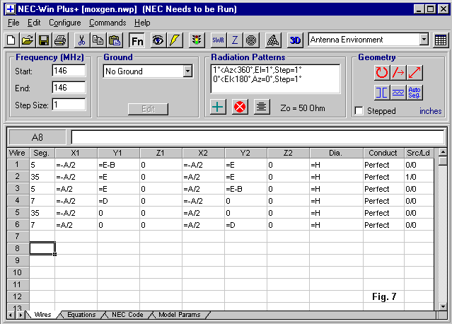
The easiest way to find out how adequate the equations are is to design a few Moxon Rectangles and then test their modeled performance. So that you can correlate the dimensions to the model description, Fig. 7 provides the variables entry version of the wires page. Note the calculated values for all X entries and the calculated values for the driver tails. In the examples, I shall show only the values version of the wires page, and you can extrapolate back to the equations page values for A through E. All dimensional values will be in inches. I have also adopted the convention of placing the reflector at Y=0.
1. A 7.15 MHz #12 wire version: The wires page for this antenna appears in Fig. 8
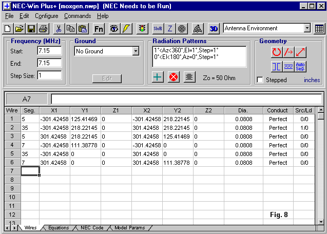
The following table gives the modeled performance for both perfect wire and for copper wire.
Frequency   Version           Gain        Front-to-Back     Feedpoint Z
MHz                           dBi         Ratio dB          R+/-jX Ohms
7.15        Perfect           6.01        39.07             53.9 + j 4.6
            Copper            5.80        31.29             55.9 + j 4.4
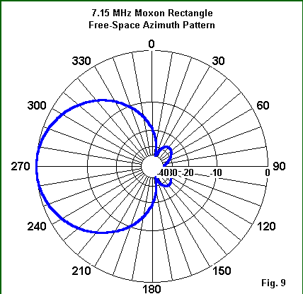
For reference, Fig. 9 shows the typical free-space azimuth pattern for a Moxon Rectangle, based on this particular model.
Because AWG #12 wire is only 0.0808" in diameter, the efficiency of this antenna drops to 96.1% as we move from perfect wire to copper wire. The losses not only show up in the additional 2 Ohms in the feedpoint impedance, but as well in decreased gain and front-to- back ratio.
Despite these facts about the wire Moxon Rectangle, the calculations yield a design that is within original modeling limits set for this exercise, with a remnant reactance of only about 4.6 Ohms.
2. A 28.5 MHz 1" tubing version: Fig. 10 contains the wires page dimensional values for the calculated model.
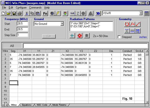
The following table lists the performance using perfect wire and aluminum tubing:
Frequency   Version           Gain        Front-to-Back     Feedpoint Z
MHz                           dBi         Ratio dB          R+/-jX Ohms
28.5        Perfect           5.97        36.89             52.9 - j 2.5
            Aluminum          5.96        36.43             53.0 - j 2.5
Despite the greater losses of aluminum relative to copper, the larger surface area of the 1" material and the higher frequency (which makes the diameter a larger fraction of a wavelength) yield a very high efficiency: 99.97%. Hence, the differential between perfect wire and large aluminum tubing is negligible. Once more, the calculated dimensions of the antenna come very close to matching the modeling limits, with only a 2.5-Ohm remnant reactance.
3. A 146 MHz 0.125" rod version: Fig. 11 shows the relevant wires page for this model.
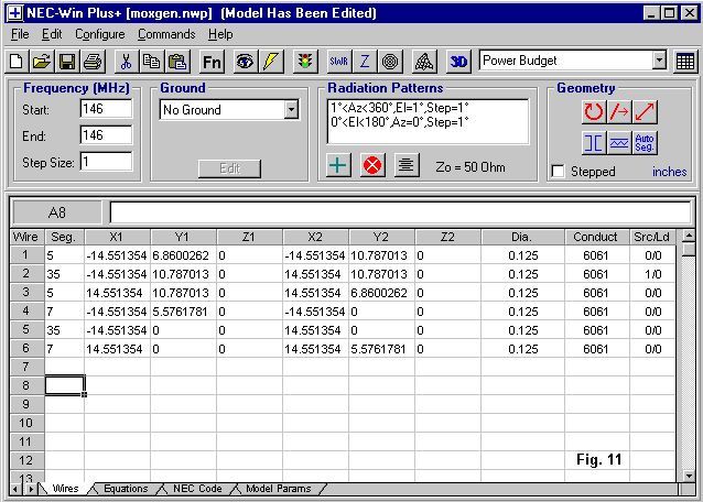
The following table lists the performance using perfect wire and aluminum rod:
Frequency   Version           Gain        Front-to-Back     Feedpoint Z
MHz                           dBi         Ratio dB          R+/-jX Ohms
146         Perfect           6.01        43.50             51.8 - j 3.4
            Aluminum          5.96        39.68             52.3 - j 3.5
The aluminum version of the antenna has a 99.1% efficiency. Although the frequency is roughly 5 times higher than the 10-meter model, the rod is only 1/8 the diameter of the 10-meter material: hence, the slightly lower efficiency. Once more, the calculated model falls well within the requirements for the goal of producing a design that can be translated directly into a constructed antenna.
Conclusion
The goal of the exercise was to develop a series of equations that one might use to design Moxon Rectangles for any reasonable frequency using any reasonable wire diameter. The equations make use of the common log of the wire diameter and the design frequency to determine the dimensions for the antenna, based upon a base-line data set of models optimized for maximum front-to-back ratio and about 50 Ohms feedpoint impedance at the design frequency. However, the equations apply only to uniform-diameter elements. The use of stepped diameter elements would require optimization within NEC-4. Since the elements are not linear, the Leeson corrections built into some commercial implementations of NEC-2 will not operate. A version of MININEC might also be used if (for the public domain version) the elements are length-tapered toward the 4 corners of the array.
Regression analysis proves a very usable technique of developing working equations for the design exercise, although the equations themselves have no theoretical significance other than fitting curves to a data set within the limits of that set. The equations can be packaged in utility programs--such as the little exercise in Basic--or they can be applied directly to a NEC model within a program capable of modeling by equation.
For those interested in modeling by equation, the model shown here is available in .NWP format at the Nittany Scientific (web.archive.org) website, along with some other models using equations featured in the monthly Antenna Modeling column. Also see the Antenna Modeling Programs page.
A stand-alone Windows program that calculates the dimensions of a Moxon rectangle for a near-50-Ohm feedpoint impedance, as described in "Designing Moxon Rectangles by Equation and by Model," has been developed by Dan Maguire, AC6LA. You may obtain a free copy from his web site: www.ac6la.com/moxgen1.html. The program will also create a model in .EZ format for use with EZNEC or in .NEC format for use with NEC-Win software or with generic NEC programs. The only required input entries are the design frequency and the diameter of the wire or tubing to be used. Dan's site also contains a number of other very useful programs for modelers and others interested in antenna design and analysis.
An online Moxon Rectangle Calculator is also available on this site.
The quest for magic formulas for cutting antennas only futilely chases after super-simple equations using only a constant and the operating frequency. Most antenna types answer better to collections of equations based on both wire size and operating frequency. Although the equations themselves may not be simple, one can put them into packages that are simple to use. However, easy generation of building dimensions is no substitute for understanding the fundamentals of how such antennas work.
Note: I am indebted to the work of Lee Lumpkin, WB8WEV, and Barbara Craig, KC8KJA, whose initial regression analysis work on some of my #14 copper wire Moxon models convinced me that a more general solution to Moxon Rectangle design was possible. Dan Hendelsman, N2DT, also deserves thanks for leading me to shareware regression analysis software.
Updated 06-12-2002. © L. B. Cebik, W4RNL. The original item appeared in AntenneX for September, 2000. Data may be used for personal purposes, but may not be reproduced for publication in print or any other medium without permission of the author.