
 From Two to One
In the preceding two episodes, we examined clusters of options for vertical and horizontal bi-directional wire arrays based on the dipole as the root antenna. Each cluster only sampled the options available, and we might easily add to the number of clusters. However, our goal was to present each cluster in an internally consistent environment to ease some of the difficulty in decision-making. Within each group, the individual can now use consistent performance data in combination with dimensional data, installation challenges, and budgetary cautions when deciding on the next antenna to build.
Very early on, a perennial question arose: how does one convert a bi-directional array into a directional beam? Once more, we have options. Most handbooks treat the options in different chapters, so we rarely receive any kind of overview of available techniques. Although our space is small and therefore our samples will be few, we can partly correct the oversight.
Consider two elements of similar size, at least one of which would serve as a bi-directional antenna. To create a directional end-fire beam from these two elements, we have to provide each element with the correct relative current magnitude and phase angle to yield the strongest possible forward lobe and the weakest possible rearward lobe. Similar considerations apply to both multi-element arrays and to large collinear arrays. As a convenience in sorting out how we accomplish the goal, we can separate the techniques into 4 general groups: parasitic methods, phasing methods, screen reflection, and traveling-wave termination. Not all techniques are equally apt to all antenna types and situations, but all have a place in the option set.
Parasitic Methods
Many hams associate parasitic elements almost solely with Yagi-Uda arrays based on the half wavelength antenna element. However, designers have long realized that parasitic elements will work with almost any bi-directional antenna. A parasitic element approximates the conditions that we may achieve directly by complex phasing systems, but it does its work solely by virtue of its length, diameter, and spacing from the original element. For a given spacing and diameter, if we shorten an element relative to the original one with a feedpoint (now called the driver), the new element will show a negative relative phase angle for its current and the main forward lobe will form in its direction. It has become a director. If we lengthen the element relative to the driver, then its current will show a positive phase angle relative to the current on the driver and the main forward lobe will be in the direction of the driver. The new element has become--by convention--a reflector. Reflector-driver arrays tend to show a wider operating bandwidth but poorer gain and front-to-back characteristics than optimized driver-director arrays. Hence, reflector-driver arrays are easier to tame, that is, easier to field-adjust into acceptable performance. We may fairly use these basic principles of parasitic element operation to create a large variety of directional beams.
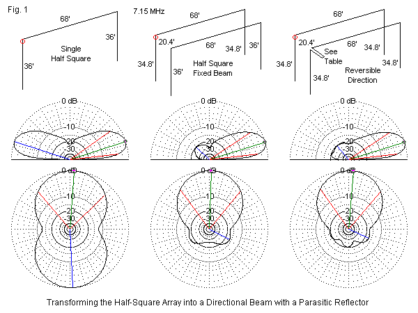
Consider the half-square array, essentially a broadside array consisting of 2 vertical dipoles in an easily reproduced wire antenna. See Figure 1. The sketch shows the single half square along with 2 parasitic variations. The dimensions differ slightly from those used in our first array episode to yield a near-50-Ohm feedpoint impedance. However, we are still using AWG #12 copper wire, average ground, and a maximum height of 50'. The left-most plot shows the azimuth pattern with its slight misalignment due to the corner feedpoint. Table 1 supplies the modeled data.
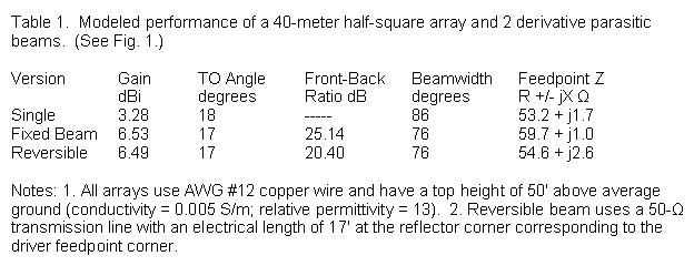
We may add to the original array a reflector and optimize the vertical lengths for maximum front-to-back ratio with the selected spacing. The forward gain increases by about 3.2 dB with only a small narrowing of the beamwidth. The 180° front-to-back ratio is excellent. The rearward quartering lobes show a very slight imbalance, but not to a point of creating problems in using the array. The structure is very simple to replicate, and the feedpoint impedance remains "coax-ready."
Rather than lengthen the reflector physically, we may also lengthen it electrically. One convenient method is to use a shorted length of transmission line to add to a driver-length element enough inductive reactance to create an effective reflector element. The sample uses 50-Ohm line at an electrical length of 17'. Suppose now that we add such a length (adjusted physically for the velocity factor of the selected coax) to the driver and bring it to a central point between the elements. We can install a remotely operated switch that converts one side into just an extension of the feed cable and the other side into the required shorted-stub. (Use a DPDT switch or relay to isolate the braids as well as the center conductors.) We now have a reversible half-square beam with virtually the same gain as the fixed version and a very useful rearward lobe set. The need to place the load and the feedpoint on the same side of the array creates a bit more imbalance in the pattern, but nothing fatal to the array's use.
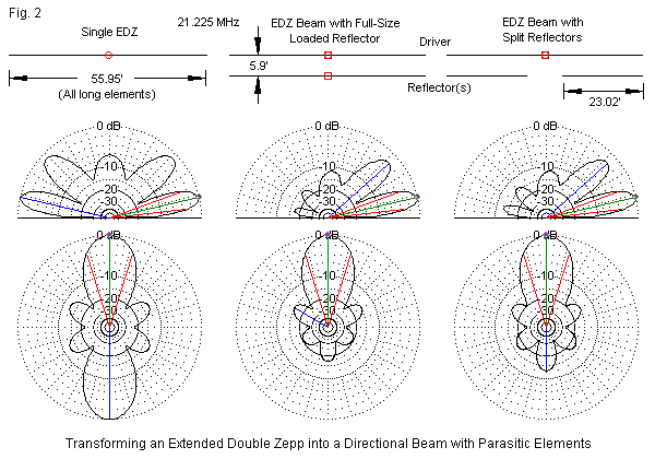
We can also apply parasitic methods to collinear arrays, for example, the extended double Zepp (EDZ) shown in Figure 2. The sample EDZ uses a length just above 1.2 wavelength to reduce the sidelobes. Like our earlier horizontal bi-directional arrays, the sample uses AWG #12 copper wire and is 1 wavelength above average ground. Table 2 provides the modeling data for both the single EDZ and two versions of a parasitic beam.
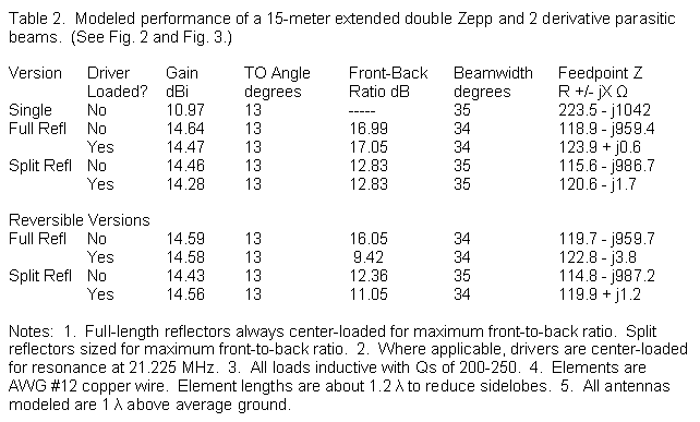
The first version uses a full-size reflector element. Since the element will be capacitively reactive, we can incorporate electrical lengthening into the center loading inductive reactance and tune the element for maximum front-to-back ratio. We also have the option of adding a coil to the center of the driven element to achieve resonance and simplify matching. For example, with the same parasitic array set for resonance, we might use a 1/4 wavelength section of 75-Ohm cable as a matching section for a 50-Ohm main feedline. Providing the driver with inductive reactance at a normal Q range of 200 to 250 has its costs in terms of a slightly lower forward gain. However, the forward gain shows well over a 3-dB increase relative to the single EDZ element.
We may also simplify the structure somewhat by using a split reflector element, with a section for each outer half wavelength of the driver. The front-to-back ratio will not be as high as with a full-size element properly loaded, but we save the trouble of having to field adjust a reflector inductor for maximum front-to-back ratio.
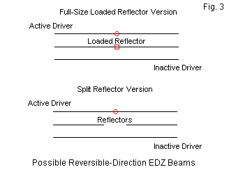
Figure 3 shows two ways of obtaining reversible EDZ beams from the same reflector options. In both cases, we find decreases in the reported data from the model in one or another performance category, as shown in the bottom lines of the table. Mutual coupling between the active and inert drivers is stronger than in the case of comparable reversible-direction wire Yagis. Nevertheless, some combination of elements may satisfy a given set of operating needs.
Phasing Methods
We often employ phasing methods to improve the rearward null performance of an array. Rarely do phasing methods show very marked gain increases over parasitic methods applied to essentially the same array. In some cases, such as the fixed half-square beam, resorting to phasing techniques would only add considerable complication for little, if any, detectable improvement. In other cases, however, phasing treatment may show marked improvement.
Phasing techniques essentially add an energy source to what we may achieve with parasitic methods. Parasitic techniques achieve the goal of setting the relative current magnitudes and phase angles to create a beam by virtue of mutual coupling between the elements. A driver-reflector Yagi, for example, rarely surpasses 12-dB front-to-back ratio. If we phase feed the two elements, we can create current magnitude and phase relationships that can easily raise the front-to-back ratio to 20 dB. Indeed, if we are willing to sacrifice some gain, we can create 180° front-to-back values as high as 50 dB--but only for the narrowest of bandwidths.
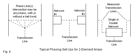
Many hams have a restricted view of phasing techniques. ON4UN's Low-Band DXing has perhaps the largest collection of practical phasing techniques. We may usefully but incompletely categorize the techniques into 3 groups, as shown in Figure 4. On the left are methods that use transmission-lines to achieve the requisite splitting of current and transforming the current magnitudes and phase angles to optimal values. The ZL-Special technique of using a single 1/8 wavelength line with a half-twist misled many builders into believing that line impedance transformation was the critical factor. However, the rate of current transformation along a line may not coincide with the impedance transformation. Particular set-ups of elements may require a forward, a rear, or an intermediate feedpoint. One part of the line may require a half-twist or not. Indeed, there are many situations in which available transmission lines or those we might construct simply will not provide the required current magnitude ratio and the phase angle difference that yields an effective beam.
The most direct route around this problem is to employ phase-changing networks at each element, as suggested by the middle sketch. Due to the weight of such networks, we ordinarily employ them with ground-mounted vertical monopole systems. An alternative is shown on the far right. We may employ ground-mounted networks and use measured transmission-line lengths to each element. Current undergoes a full cycle in 360° of line (not in 180°, as is the case for impedance). However, the lines may have different lengths to add additional current and phase angle transformations to the output of the network or networks.
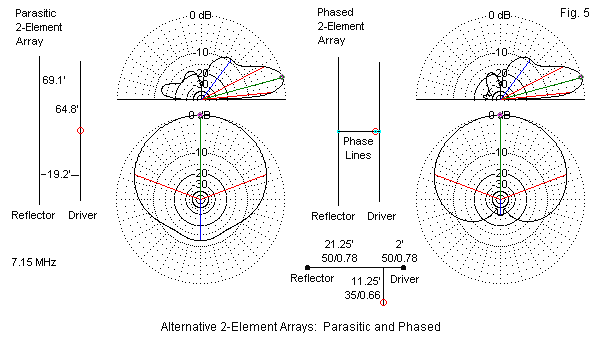
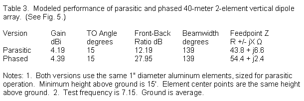
Network calculations require more space than we have for this overview, but we can demonstrate the potential benefits of a transmission-line-based phasing system with a single example. Consider 2 vertical dipoles set up for parasitic operation, as shown in Figure 5. The element center points are at equal heights, and the lowest approach to average ground for this 7.15-MHz array is 15'. With the 1" diameter aluminum elements used for the array, we obtain the patterns shown in the figure and the modeled performance figures that appear in Table 3. Like virtually all good 2-element driver-reflector parasitic systems, we obtain about 3.2-dB gain over a single vertical dipole. As we might expect from such an array, the maximum front-to-back ratio is just over 12 dB. With the element dimensions shown, the feedpoint impedance is close to 50 Ohms.
Without changing any of the array dimensions, we may improve performance, especially with respect to the front-to-back ratio, as shown on the right side of Figure 5. The required phase line has two sections. The short section goes to the forward element. The longer section goes to the rear element and uses a half twist. The phase line sections consist of a foam dielectric coaxial cable with a 50-Ohm impedance and a velocity factor of 0.78. (A 0.66 velocity factor would yield physical lengths too short to handle the spacing between elements.) The net feedpoint impedance is about 30 + j13 Ohms, hence the need for a section of 35-Ohm cable (or parallel sections of 70-Ohm cable) to yield an impedance close to 50 Ohms. The specified length entails a velocity factor of 0.66. For the effort of figuring or finding a usable phasing system, we obtain a very small increase in gain and a very large improvement in the front-to-back ratio. At the same time, we maintain a coax-ready array.
Planar or Screen Reflector Techniques
Screen or planar reflectors date back to the 1920s and the billboard array. Once considered ungainly at HF, they find extensive use in the UHF region. The reflector is largely untuned, although extensive modeling has shown that gain reaches maximum when the limits of the screen at about 0.5 wavelength beyond the limits of the driving array in all dimensions. The screen is unlike the parasitic reflector, which does not reflect but instead has a size to yield the correct current magnitude and phase angle to yield a maximized forward and a minimized rearward lobe. The screen is a reflecting surface that acts largely (but not exclusively) according to principles derived from optics.
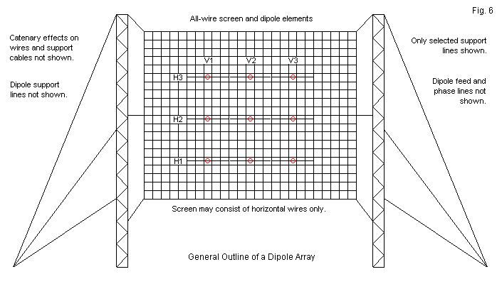
In the HF region, the short-wave broadcast industry makes extensive use of screen reflector arrays with banks of dipoles fed in phase for a main beam that is broadside to both the screen and the driving array. Figure 6 shows the outlines of a very large array consisting of 3 rows and 3 columns of dipoles. Only a few of the support cables appear in the sketch. To have shown them all would have obscured the essential electrical elements of the array. It is possible to construct far smaller screen arrays to good effect. For example, a lazy-H is a bi-directional array that corresponds to a 1V-2H scheme in terms of the designations in Figure 6. Not only would a screen that is 2 wavelengths high by 2 wavelengths wide yield a directional signal, it would produce about 5 dB gain over the maximum gain of the basic lazy-H.
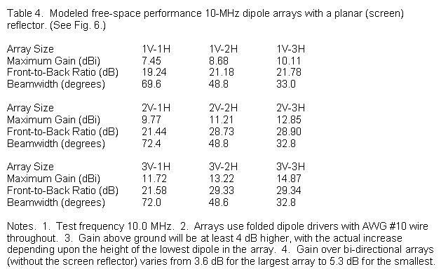
The models used to test the capabilities of the dipole array with a screen reflector use commercial standards. Commercial dipole arrays strive to be broad-banded. The wire is AWG #10 copper (although many arrays use aluminum-coated steel). A combination of folded dipoles and a spacing of 0.3 wavelength yields a wider operating bandwidth, although it produces less than absolutely maximum gain. Table 4 shows the modeled free-space performance of screened arrays from 1V-1H up to 3V-3H. Corresponding to the data entries are the azimuth patterns that appear in Figure 7. Each pattern rests on the use of a screen with dimensions optimized for the driving array size. (Commercial HF dipole arrays may skimp a bit on the screen size, and because the elements are horizontally polarized, the screen may use only horizontal wires. When a screen uses only horizontal wires, some reflector elements may exhibit parasitic properties, including high-than-normal current magnitude excursions.)
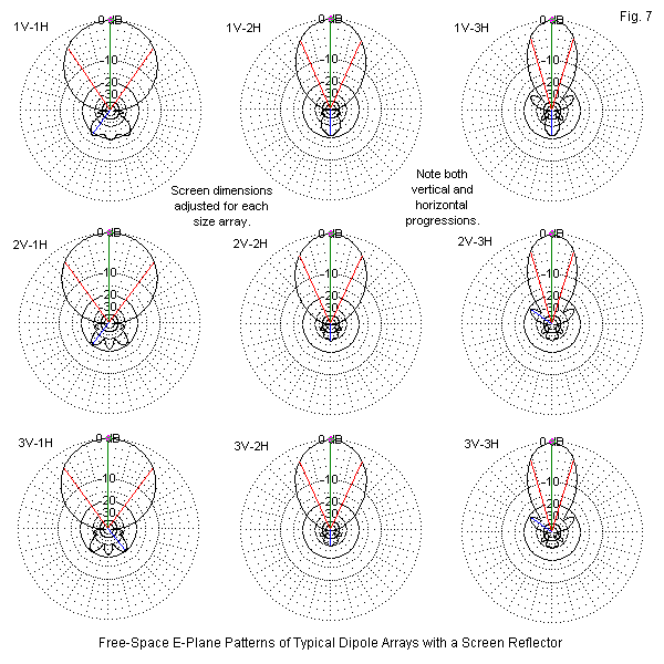
The data and patterns are notable in several different ways. As we add elements vertically, the beamwidth does not change, although for each column, we find about the same gain increase with each added vertical bay. When we read the table and the patterns horizontally, we discover that each horizontal bay that we add reduces the beamwidth and increases the front-to-back ratio. One major advantage of the dipole array is that it allows the operator to select the best compromise between gain and beamwidth just by opting for an array size. In addition, by phasing each vertical bay in equal increments (for example, 30°, 60°, 90° for a 3-bay array), it is possible to slew the signal angle with respect to the plane of the array without major distortion to the pattern shape.
In amateur use, a planar or screen reflector accepts a wide variety of drivers. The drivers may be either vertically or horizontally polarized and range from simple dipoles to more complex bi-directional arrays. Half-squares, rectangles, and side-fed quads are all applicable to a planar reflector to increase the forward gain and to yield a very good front-to-back ratio. In addition, for these single-feedpoint drivers, we can often find a spacing between the reflector and the driver that yields a desired feedpoint impedance, such as 50 Ohms, without sacrificing significant gain. One caution to observe is not to bother using an end-fire array in front of the screen. The screen will dominate so that the phased elements will not provide any significant further gain.
Traveling-Wave Termination
Long-wire technology arose in the late 1920s and more especially in the 1930s in answer to the need for very precise trans-oceanic point-to-point communications. Edmond Bruce stands at the head of the class of antenna engineers for his invention of the "king" of long-wire antennas. Although these collinear arrays have largely passed out of service as installations strive to save real estate, amateurs still dram of wire antenna farms. Indeed, one humorist from past decades once specified his ideal DX antenna as a very large rhombic installed on a rotatable island. The basic long-wire shapes are the single long wire, the V, and the diamond or rhombic. Each of these shapes is essentially bi-directional. We obtain a directional beam by adding a terminating impedance at the array end opposite the feedpoint. In doing so we convert a standing-wave antenna into a traveling-wave antenna, although the conversion is imperfect.
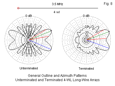
We measure the basic single long-wire in wavelengths. The sample shown in Figure 8 is 4 wavelengths long. As the patterns show, the long-wire has a split lobe. As we make the antenna longer, the lobes in each direction grow closer to the axis of the wire itself, but they never meet for almost all practical lengths. The sample long-wire antennas in these notes use 0.16" diameter (AWG #6) wire and are 1 wavelength above average ground at a test frequency of 3.5 MHz. The end-fed single wire has a lobe count that is twice the number we would expect of a center-fed wire of the same length. As the data in Table 5 show, an unterminated or standing-wave long-wire has a natural imbalance of nearly 2 dB away from the feedpoint.
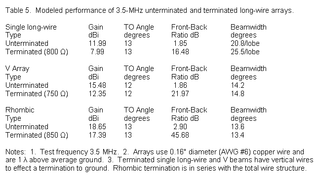
When we add a terminating impedance (in this case 800 Ohms), we obtain the directional pattern shown in Figure 8. The gain drops significantly, not only because of the terminating resistor, but as well because each end of the array must have a wire to a common ground. The two vertical lines tend partially to fill the pattern nulls and thereby prevent the array from obtaining full gain. Nevertheless, we also obtain a very wide operating bandwidth. In fact, the SWR bandwidth is significantly wider than the practical bandwidth for the pattern shape.
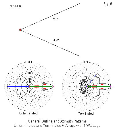
The V array in Figure 9 rests on the long-wire. The angle between the two legs is a function of the lobe angle of each leg--as shown by the lobes of the single long wire. Two lobes coincide down the centerline between lobes, resulting in a bi-directional pattern that is close to equal strength in both directions. The feedpoint is in series with the legs at their junction. If we wish to add a termination, we must run lines to ground, where we place separate terminating impedances, or we must run a line between the far ends of the V with the termination centered. In either case, we discover a decrease in gain relative to the unterminated array. However, the pattern is very strongly directional, and the SWR bandwidth far outstrips the practical operating bandwidth. With a V array, changing operating frequency changes the leg length as measured in wavelengths. Hence, the angle for an acceptable pattern has a limited frequency range of about 2:1.
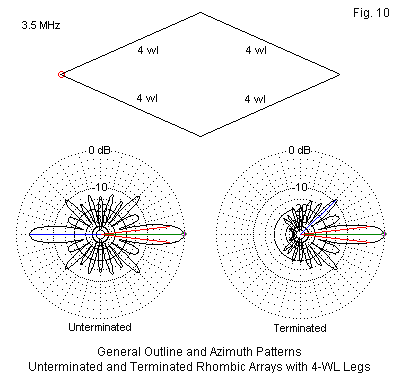
With the possible exception of VK3ATN's moon bounce 2-meter rhombic in the 1960s, I am unaware that anyone has ever bothered to use an unterminated rhombic, as shown in Figure 10. However, I have included data on it in Table 5 to compare with the far more common terminated version. A rhombic with 4 wavelength legs is, of course, twice as long overall as a V with 4 wavelength legs, but the width is about the same, since the same angle-based construction is involved. The terminating impedance of a rhombic (850 Ohms in this sample) is in series with the collinear array wires. Therefore, we see far less difference between the gain of the unterminated and the terminated versions. However, we can achieve very high front-to-back ratios.
For commercial service, the major failing of all long-wire technology was the high level of the sidelobes, clearly evident on all of the patterns. The correct V or rhombic angle might combine two or more long-wire lobes, but it did little to suppress the other lobes in the long-wire pattern. For amateur serve, optimized V-beams and rhombics have two major drawbacks. Acreage is one of them. The other is the extremely narrow beamwidth. Nevertheless, the technique of using a termination to convert a bi-directional array into a directional beam deserves its place among the options available to us.
Conclusion
These notes have taken a somewhat different approach to converting a bi-directional array into a directional beam by providing an overview of the major techniques available to us. Not every technique is applicable to every bi-directional array that we might wish to convert into a directional beam. As well, in some cases, a technique might be applicable in principle but highly impractical to implement. In most cases, however, we likely will find more than one potential method of conversion and can weigh each against the other factors (for example, complexity, finickiness, budget, etc.) that go into our final building decisions.
Updated 11-01-2006. © L. B. Cebik, W4RNL. This item first appeared in QEX, Nov/Dec, 2006, pp. 51-59. Reproduced with permission. Copyright ARRL (2006), all rights reserved. This material originally appeared in QEX: Forum for Communications Experimenters (www.arrl.org/qex).