Because the rhombic antenna, especially when terminated, offers very high gain, it has received more design attention than any of the other long-wire antennas. The straightforward basic design data sampled in Part 4 does not exhaust the significant variations on the basic configuration. One potential particularly suited to amateur service in the upper HF range is the possibility of operating a rhombic over a 2:1 frequency range, thus allowing coverage of 20 through 10 meters. We shall examine one tried and true design and try to find out the basic design premise that allows it to be successful.
When an antenna is good at what it does, we can count on efforts to make the good even better. For narrow-beamwidth point-to-point communications, the rhombic is very good. One very old technique to improve performance somewhat is the use of multiple wires in each side of the rhombic. They come together at the feedpoint and at the terminating resistor end, but spread vertically where the facing Vs are widest. Some claims about the technique will prove correct, such as the addition of a small increment of gain. However, other claims may turn out to have other foundations than the use of multiple wires.
Finally, we shall address an interesting technique for further suppressing the remnant sidelobes in the rhombic radiation pattern. Laport developed a scheme for using closely spaced rhomboid structures in parallel. The centerlines for each of the independent rhomboids fed in parallel are offset from each other. The technique will offer a small gain advantage over the single-wire rhombic, but will reduce sidelobes by a very significant amount.
Although these developments are worth our notice here, they will not exhaust the variations on the rhombic. There is, for example, the so-called half-rhombic, consisting of one side of a rhombic played against ground. Unfortunately, lossy soil does not permit the antenna to play like a true rhombic, due to ground reflections and losses. Despite its name, the antenna operates more like a terminated, end-fed, inverted V, and highest performance occurs with only a slight elevation of the centerpoint above ground. The antenna appears in Bruce's 1931 article and he calls it simply an inverted-V. The name "half-rhombic" came later from other builders. Other variations on the rhombic have emerged in answer to specific commercial and governmental communication needs. The result has been highly complex arrangements of wire structures well beyond the scope of these introductory notes. Nevertheless, the variations that we have selected should provide a sufficient foundation to let you examine the classical literature on advanced rhombic designs with understanding.
Multi-Band Rhombics
Although we have briefly mentioned multi-band use of long-wire antennas, we have not paused long to investigate their performance in broadband service. We shall rectify this situation, if only briefly, by looking the ARRL rhombic intended for upper HF service from 14 through 28 MHz. The antenna first appeared in The ARRL Antenna Book somewhere between 1965 and 1974, and has been a prime example in the book's treatment of traveling-wave antennas. Fig. 1 shows the general outlines of the antenna.
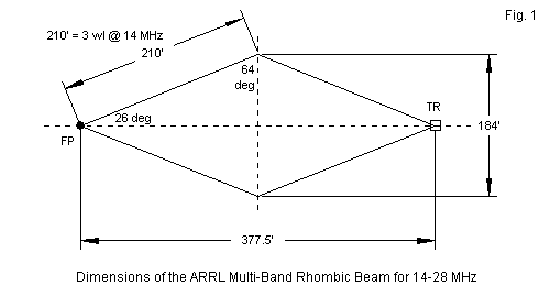
One notable feature of the antenna is that its design emerged long before modeling software became available. Hence, its outline rests directly on the original rhombic design equations, as filtered into design nomographs. The design begins with 3 wavelength legs at 14 MHz along with a height of about 70' or 1 wavelength at the lowest frequency of use. It uses a prescribed tilt angle of 64 degrees and hence an angle A value of 26 degrees. These values coincide perfectly with the values developed via computer modeling. For this model, I followed the typical amateur conventions and used a 600-Ohm termination and an SWR reference impedance of 600 Ohms. The following table lists the modeled performance of the antenna over the 5 amateur bands between 14 and 28 MHz.
Modeled Performance of the ARRL Upper HF Rhombic with a 600-Ohm Termination
Frequency MHz      14.0        18.118      21.0       24.94      28.0
Parameter
Gain dBi           16.04       17.89       18.38      18.31      17.33
El. Angle deg      14          10          9          7          6
Front-Back dB      19.93       15.28       24.68      15.27      32.12
Beamwidth deg      17.0        13.0        10.8       8.6        7.0
600-Ohm SWR        1.25        1.79        1.22       1.65       1.22
The gain values parallel almost exactly the curves in Fig. 8 in Part 4, which is also for a rhombic with 3 wavelength legs and an angle A of 26 degrees. The three differences between the earlier model and the present one are the design frequency (3.5 vs. 14 MHz), the wire (perfect 0.16" vs. copper AWG #12 or 0.0808"), and the terminating resistor value (850 vs. 600 Ohms). Fig. 2 shows a gallery of elevation and azimuth patterns at each of the test frequencies. Note that this gallery differs from the galleries in the earlier parts of this series because angle A is optimized in combination with the leg length only at the lowest operating frequency.
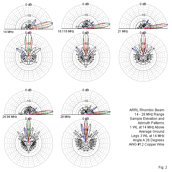
The sidelobe structure (including the rear-most lobe) of the patterns for frequencies above 14 MHz does not parallel any of the patterns in the earlier galleries (Fig. 9 in Part 4, for example) because angle A (and the tilt angle B) remain constant while the leg length changes as a function of the ever higher operating frequency. As a result, we find lobes that do not appear in the main gallery of optimized designs for each leg length. They result from incomplete cancellations that occur with a non-optimal combination of leg length and angle A. As well, the use of the relatively low terminating resistor value (600 Ohms) results in a set of SWR values that approximates those shown for the frequency sweep in Fig. 6 of Part 4.
The ARRL rhombic design nevertheless shows itself to be a very competent performer over its 2:1 frequency range. It captures perhaps the key element in multi-band rhombics: optimize the design for the lowest anticipated frequency, accounting for both antenna height and anticipated leg length. As the frequency increases, the gain will rise, as indicated by 2 of the leg-length equations early in Part 4. According to those equations, peak gain would occur somewhere close to 15 meters. With a satisfactory terminating resistor, the antenna will perform quite well over a 2:1 frequency range. With a higher value than 600 Ohms, the SWR curve would smooth out more completely, if we use a reference impedance to match the termination (and hence a feedline with a higher characteristic impedance than 600 Ohms).
The general procedure has exceptions. For example, the idea of optimizing the rhombic at the lowest frequency in the 2:1 requires careful selection of the value of angle A. If we increase the angle in order to raise the gain at the lowest frequency, we shall find that we have limited the operating frequency range upward. The gallery of azimuth patterns shows that, at 28 MHz, the innermost sidelobes are almost as strong as the main lobe. If we select a maximum gain value of angle A for 14 MHz, the 10-meter pattern will show 3 lobes, and the lobe that is on-axis with the array will no longer be the strongest. Such a condition defeats the main goal of creating a rhombic in the first place: the desire to achieve point-to-point communications on a heading in line with the two acute angles of the rhombus. If we reduce the value of angle A at 14 MHz, then the main lobe broadens with a loss of gain. For the selected height, the ARRL rhombic antenna selects a value of angle A at 14 MHz that yields roughly equal gain on both 20 and 10 meters, which is generally a good selection for amateur service. It also illustrates why much of the classical rhombic literature recommends no more than a 2:1 frequency range for the antenna, even though the range of acceptable matching is much wider.
Multi-Wire Rhombics
Perhaps the most common variation on the single-wire rhombic beam involves the use of multiple wires running from the feedpoint to the terminating resistor on each side of the centerline. The added wires join the level wire at both the feedpoint and the terminating resistor. However, they spread above and below the level wire at the widest points in the array. In general, the wires are the same length as the level wire, theoretically resulting in the wires being further offset from any support post toward the centerline. However, the amount of differential is a very small fraction of the total wire length along each leg, and allowing the spread wires to be slightly longer in order to align the supports will create no performance problems.
In order to model the multi-wire rhombic, using 3 wires as a sample version, we must alter the means by which we create the antenna geometry. The left side of Fig. 3 shows the method used in Part 4. It consists of only 4 wires per rhombic, with a split source and a split load. At the source end, we simply place a source on each of the segments adjacent to the wire junction. Since they are in series, the feedpoint impedance is the sum of the source impedance values reported for each source. The split load simply creates a balance at the far end of the array by placing a load resistor on each of the wire segments adjacent to the junction. The overall terminating resistor value is simply the sum of the 2 load resistance values. To use a real example from the last episode, the 4 wavelength-leg version of the terminated rhombic used legs that are 4.00 wavelengths long. The distance from centerline to a side peak is 1.563 wavelengths, while the distance from the midline to either end junction is 3.682 wavelengths. The resulting angle A is 23.0 degrees, and the overall rhombic length is 7.364 wavelengths.
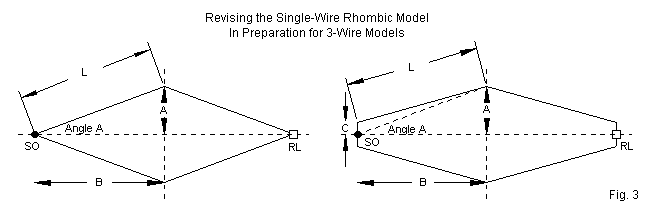
The "pointy" ends of the model do not permit ready feeding for a multi-wire version of the antenna. Therefore, we must revise the modeling system to allow the wires to terminate together for a common feedpoint and for a common load resistor. The right side of Fig. 3 shows the general technique. We create a flat or blunt end at each rhombic point. To ensure that the source segment has adjacent segments of equal length on each side, we make the blunt end-wires 3 segments long. So that the wires will have segments as close as possible in length to the segments in the long side wires, the blunt end wires are 0.14 wavelength, based on the use of 20 segments per wavelength in the side wires. Now let's set the total length of the rhombic to 7.36 wavelengths, with a 3.68 wavelength distance from either end to the midline. The distance from the centerline to the peaks will be 1.56 wavelength. The angle (A) from the centerline to a peak will be 22.97 degrees. However, the overall wire length will not be exactly 4.0 wavelengths. Instead, the sloping portion of the side wire will be 3.97 wavelengths, added to half of the blunt end-wire (0.07 wavelength) for a total length of 4.04 wavelength. All figures are for rhombics 1 wavelength above average ground with lossless 0.16" wire at 3.5 MHz.
I have recorded seemingly insignificant variations in models because these variations do create differences in the reported performance of the antennas. The following table explores the performance of the 4-wire "pointy" version of the antenna using various terminating resistor (RL) values.
Performance of a Pointy Single Wire Rhombic with 4-Wavelength Legs and Various Terminating Resistors
Terminating          Maximum         Front-Back         Feedpoint Z
Resistor (Ohms)      Gain dBi        Ratio              R+/-jX Ohms
 600                 17.30           18.07               737 - j 40
 700                 17.28           23.13               793 - j 13
 800                 17.27           33.22               844 + j 14
 850 *               17.27           43.97               869 + j 27
 900                 17.28           32.75               892 + j 41
1000                 17.29           24.29               936 + j 67
1100                 17.30           20.40               977 + j 94
1200                 17.32           17.94              1015 + j120
We should note 2 special items in this table. First, the starred item represents the version of the antenna selected for inclusion in the larger table in Part 4. There are 2 reason for selecting this terminating resistor value. It does result in the highest front-to-back ratio, although this reason is secondary to another. Without becoming too finicky, the load resistor and the resistive component of the feedpoint impedance are most closely matched. With smaller values of terminating resistance, the resistive component of the feedpoint impedance is always higher than the load resistance. For all terminating resistors larger than the selected value, the feedpoint resistance is always lower than the terminating resistance. Since a terminated long-wire antenna operates in a similar manner to a transmission line, matching the load resistance to the feedpoint resistance results in the widest SWR bandwidth when referenced to the load resistance value. The required value does not change with changes in the leg length so long as the angle A is selected to align the lobes for maximum gain. However, it will change with even small departures from the ideal geometry. It will also change with the height of the antenna above ground and with the quality of the ground itself, since both of these factors will change the effective impedance of the antenna when viewed as a length of transmission line.
Second, note the remnant inductive reactance in the feedpoint impedance. The reactance is inductive. One traditional reason for using multiple wires in the rhombic legs is that it introduces a compensating capacitive reactance due to interactions among the wires. A capacitive reactance represents--with respect to feedpoint impedance--a slight electrical shortening of the antenna circumference. Wire interaction is unnecessary to explain the electrical shortening of the overall rhombic loop. All closed loops of a preset total circumference become electrically shorter if we increase the wire diameter--exactly the opposite effect of fattening elements in open-ended elements. Since the 3-wire rhombics will have effectively a fatter element, even though variable in equivalent diameter along the leg lengths, the loop will become electrically shorter and thus show a more capacitive reactance at the feedpoint.
The blunt-end version of the 4 wavelength-leg rhombic makes only one change among the factors that tend to affect the optimal value of load resistance: the geometry. The shape changes are very small overall, but they do have consequences, as shown in the following table that parallels the one for the pointy version of the same rhombic.
Performance of a Blunt Single Wire Rhombic with 4-Wavelength Legs and Various Terminating Resistors
Terminating          Maximum         Front-Back         Feedpoint Z
Resistor (Ohms)      Gain dBi        Ratio              R+/-jX Ohms
 600                 17.40           15.26               806 + j121
 700                 17.37           18.48               857 + j 81
 800                 17.35           22.87               903 + j 41
 900                 17.35           30.23               945 + j  2
 975 *               17.35           38.04               973 - j 27
1000                 17.35           35.88               982 - j 37
1100                 17.36           26.68              1016 - j 74
1200                 17.38           22.27              1046 - j110
The closest match between the terminating resistor and the feedpoint resistance occurs with a value of about 975 Ohms. The difference between the 2 models of 125 Ohms may seem significant, but it is likely that construction variables would wash out the difference in terms of trying to determine which model better captures a physical rhombic with 4 wavelength legs at a height of 1 wavelength above average ground. As well, small changes in the segmentation per wavelength will also change the reported values somewhat. Note also that the progression of inductive to capacitive reactance is the reverse of the pointy geometry. Nevertheless, the pattern of the feedpoint resistance remains: below the optimal load resistance, the feedpoint resistance is higher than the load resistor and above the optimal load, the feedpoint resistance is less than the load resistance.
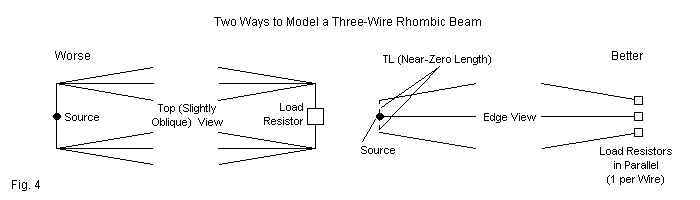
The blunt-end version of the modeled 4 wavelength-leg rhombic will become the standard against which we measure 3-wire rhombics using the same leg length. However, modeling the 3-wire rhombic presents another modeling challenge of its own. Theoretically, the wires must join on each side of both the feedpoint wire and the load resistance wire. The relevant modeling sketch of this situation appears on the left in Fig. 4. There is a difficulty built into this scheme. Because the wires are not widely spaced relative to their length, the segments at the junction interpenetrate for a considerable distance along the segment length. Even though the level of inter-penetration may not reach a level that raises flags within NEC, it may still be sufficient to alter the performance reports of the array, since the inter-penetration does affect NEC's current calculations.
To test the model, let's explore what happens as we pass the model through a number of loading resistor values. The side wire expansion is very modest, reaching only 0.0125 wavelength at the midline. That distance amounts at 3.5 MHz to about 1.06 m or 3.49', with an antenna that is over 630 m (2068') long. Like all of the models, the 0.16"-diameter wire is lossless and the wires are 1 wavelength above average ground.
Performance of an Angled 3-Wire Rhombic with 4-Wavelength Legs and Various Terminating Resistors
Terminating          Maximum         Front-Back         Feedpoint Z
Resistor (Ohms)      Gain dBi        Ratio              R+/-jX Ohms
 600                 18.92           16.76               795 + j335
 700                 18.92           18.57               834 + j319
 800                 18.92           19.64               870 + j305
 900 *               18.93           19.68               902 + j291
1000                 18.94           18.96               933 + j278
1100                 18.95           17.93               961 + j266
1200                 18.96           16.87               987 + j255
Although we are not yet positioned to evaluate the gain improvements, the impedance column should give us pause. The very large rise in inductive reactance relative to the blunt single-wire model exceeds what we might otherwise reasonably expect from adding 2 wires with fairly narrow spacing relative to the frequency. In addition, the indicated "ideal" termination resistor value (900 Ohms), does not coincide with long-standing empirical experience, which suggests a value closer to 600 Ohms.
We may reformulate the model using some techniques that have proven useful with quad loops and similar structures. The right side of Fig. 4 outlines the techniques at each and of the antenna. At the feedpoint end, we prevent the wires from meeting, but bring them to a 0.001 wavelength spacing (about 86 mm or 3.4"). Next, we create a bridge wire for each loop. The source excitation goes to the center (level) wire on the middle segment of the bridge wire. From the corresponding segments on the upper and lower section, run 600-Ohm transmission lines to the source segment. The impedance is not critical, because the lines will be only 0.000001 wavelength long, a number that the modeler specifies in the transmission line entry. Hence, the three wires have a common source in parallel, while preventing the inter-penetration of any wires.
The termination end of the beam uses the same modeling technique of bringing the wires close (0.001 wavelength) but not allowing them to touch. We cannot create a single parallel connection using the transmission line technique, because any load resistor would be in series with the line and hence outside it. Instead, we provide each bridge wire with a load resistance that is 3 times the desired terminating resistor value. If we run the same tests on the reformulated model, we obtain the results in the following table. Note that the actual terminating resistance values are 3 times the value in the table, but occur on 3 bridge wires.
Performance of a Separated 3-Wire Rhombic with 4-Wavelength Legs and Various Terminating Resistors
Narrow (0.0125-Wavelength) Maximum Wire Separation
Terminating          Maximum         Front-Back         Feedpoint Z
Resistor (Ohms)      Gain dBi        Ratio              R+/-jX Ohms
 400                 18.60           17.14               586 + j 22
 500                 18.60           22.29               619 - j  4
 600                 18.60           31.34               648 - j 32
 650 *               18.61           36.44               662 - j 37
 700                 18.61           31.37               675 - j 42
 800                 18.63           24.01               695 - j 73
 900                 18.64           20.33               714 - j 95
1000                 18.66           18.02               733 - j105
The gain improvements over the single-wire model are more modest: about 1.3 dB. The rounded ideal load value comes very close to matching the feedpoint resistance and also corresponds to the highest 180-degree front-to-back ratio value. As expected, the capacitive reactance is slightly higher than for the blunt single-wire model, but only slightly so, since the average wire-diameter increase for the closed loop is not great as a function of a wavelength. Finally, the selected terminating load and feedpoint impedance tend to match reasonably with reported experience with these types of rhombic beams.
Most amateur rhombics cover the upper HF spectrum, and the spacing used at these frequencies is 3' to 4'. Therefore it seems prudent to test our 3.5 MHz model with a wider spacing than the 0.0125 wavelength used in the initial model. Using the same loop separation techniques, I increased the spacing at the midline to 0.025 wavelength (about 2.1 m or 7'). All other modeling parameters remain constant. The results appear in the following table.
Performance of a Separated 3-Wire Rhombic with 4-Wavelength Legs and Various Terminating Resistors
Medium (0.025-Wavelength) Maximum Wire Separation
Terminating          Maximum         Front-Back         Feedpoint Z
Resistor (Ohms)      Gain dBi        Ratio              R+/-jX Ohms
 400                 18.74           17.46               597 + j 26
 500                 18.74           22.45               629 + j 10
 600                 18.74           30.19               656 + j  7
 650 *               18.75           33.08               669 - j 11
 700                 18.75           30.20               682 - j 15
 800                 18.76           24.04               701 - j 55
 900                 18.78           20.56               721 - j 63
1000                 18.79           18.30               739 - j 71
As one might expect, by enlarging the average wire diameter by a significant amount, the gain reports increase by a very small but numerically noticeable amount. More telling is the array of front-to-back values. The peak value does not reach the level attained by the narrower 3-wire array, and that value, in turn, did not reach the peak value of the single wire blunt-end rhombic beam. However, the wider 3-wire array shows a smaller fall-off in front-to-back value as we vary the terminating load across the same range as used with the narrower 3-wire version. Compare values for this antenna with 600-Ohm and with 1000-Ohm loads with the corresponding values for te narrow 3-wire rhombic.
The near-ideal load resistance remains unchanged at 650 Ohms or thereabouts. However, the capacitive reactance at that load value is not as great as with the narrow 3-wire rhombic. The important data on the reactance is not its value at the ideal load resistance so much as it is the total range of reactance across the total set of load resistors. The narrow 3-wire rhombic shows a range of 162 Ohms, while the medium spacing (twice the narrow spacing) reduces the range to 134 Ohms--for the same set of load values.
Let's increase the maximum wire spacing at array midline one more time. We shall again double the spacing to 0.05 wavelength (about 4.3 m or 14.1'). All other parameters remain the same. Each outer leg is now about 0.0003 wavelength longer than the level center wire--about 1". With all other model parameters unchanged, we obtain the following table of modeled values.
Performance of a Separated 3-Wire Rhombic with 4-Wavelength Legs and Various Terminating Resistors
Wide (0.05-Wavelength) Maximum Wire Separation
Terminating          Maximum         Front-Back         Feedpoint Z
Resistor (Ohms)      Gain dBi        Ratio              R+/-jX Ohms
 400                 18.88           17.79               607 + j 59
 500                 18.88           22.46               638 + j 37
 600                 18.89           28.31               664 + j 23
 650 *               18.89           29.64               676 - j 10
 700                 18.90           28.16               686 - j 14
 800                 18.91           23.71               707 - j  9
 900                 18.92           20.62               724 - j 38
1000                 18.93           18.50               738 - j 56
Once more, we find the small improvement in gain, which is now about 1.5-dB higher than the blunt single-wire array. The peak front-to-back ratio continues to diminish, but the values with a 400-Ohm and with a 1000-Ohm load are higher. The curve--as we might expect for increasing wire diameter--has less of a sharp peak and covers a broader range with higher values. Although I might have increased the ideal terminating resistor to 700 Ohms, continuing to use the 650-Ohm value allows us to see the other curve changes more easily. The reactance range has shrunk to 96 Ohms total. The anomalous value for the 800-Ohm terminating resistor is accurate to what NEC reports. It may be a function of secondary effects that the other tables do not show given the 100-Ohm increment in terminating resistor values.
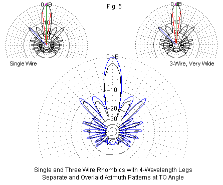
The use of 3-wires, whatever the spacing, does not change the essential elements of the rhombic pattern. Fig. 5 compares the patterns for the blunt single-wire model and for the widest 3-wire model in both separate patterns and with an overlay. The overlaid patterns show the comparative raw gain of each lobe. The separate pattern establishes that there is no essential change in the relative strength of the lobes. The only exception, of course, is the 180-degree lobe.
Amateur lore on rhombic antennas suggests that the 3-wire design may be capable of a smoother SWR curve across a broad passband than a single wire model. That lore tends to neglect the need to match the terminating resistor to the feedpoint impedance--and that impedance to the characteristic impedance of the feedline. To test this way of looking at the impedance question, I ran each of the 4 main blunt models through an SWR sweep from the design frequency to twice that frequency (3.5 to 7.0 MHz). The single-wire blunt model used a 975-Ohm SWR reference impedance, while the 3 3-wire models used a 650-Ohm reference impedance. The result appear in Fig. 6.
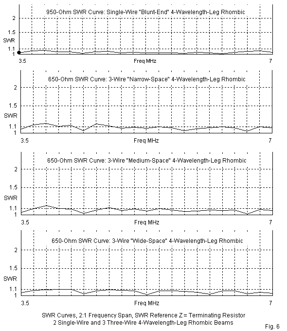
In practical terms, we have no way to make a selection among the antenna models. All 4 curves remain below 1.2:1 relative to their reference impedances across the entire range. Any device capable of broadband impedance transformation at the desired ratio would operate under very low-loss conditions. The exercise, however, does show one interesting fact: none of the 3-wire models improves upon the blunt single-wire model SWR curve. The only advantage shared by the 3-wire models is that they may better use a commercial 600-Ohm parallel transmission line than the single-wire model. However, a 975-Ohm line requires more patience than skill to fabricate in one's own shop.
The 3-wire rhombic, then, has 3 advantages over a single-wire rhombic. First, the gain improvement is real, but might not be sufficient to be noticeable in practice. Second, from a practical perspective, the ideal conditions for a 3-wire rhombic--at least one that is 1 wavelength above average soil--yield a terminating resistor and feedpoint impedance that more nearly coincides with off-the-shelf components. (Note: this result applies only to the subject antenna and requires verification for any variation in height and soil condition.) Third, the "fat-wire" effect of using wider spacing gradually widens the operating curves of some operating parameters.
Besides mechanical complexity, the 3-wire rhombics have only one almost insignificant down side. The front-to-sidelobe ratio shows a very small but steady decline as we increase the effective wire diameter. Between the blunt single-wire model and the widest 3-wire model, the decline is only about 0.2 dB. However, it appears to be a real phenomenon and runs counter to the design goals of many rhombic designers. The design goal of reducing rhombic sidelobes leads us to the third of our bits of unfinished business.
Multi-Element Rhombics
Rhombic development persisted long after its primary period of HF service in the 1930s and 1940s. With the advent of commercial broadcast VHF television in the 1950s, followed by UHF television in the 1960s, engineers searched for wide-band antennas with high gain to satisfy consumer needs in fringe reception areas. In this period, Laport published his work on the adaptation of the rhombic for this and other services. The sidelobes for a single rhombic with an overall length of about 5 wavelengths were down less than 10 dB, a situation that made the antenna susceptible to multi-path ghosting and other forms of interference. Laport's solution to the problem was to develop a dual rhombic antenna with offset axes.
Laport's dial offset rhombic is a variant of the basic idea of using two rhombics of different sizes, each with its own terminating resistor. Only certain combinations of rhombics are eligible for such use. The main criteria is that the sidelobes of one size align closely with the side nulls of the other. The result is a significant decrease in the net sidelobe strength. The combination of a rhombic with 3.5 wavelength legs and one with 6 wavelength legs provides a prime candidate for dual rhombic service. We can shorten the overall length of the combination by combining one leg from each rhombic on each side of a pair of rhomboids. The dual offset rhombic offered higher gain and greater sidelobe suppression. Fig. 7 shows both the general outline and the critical dimensions.
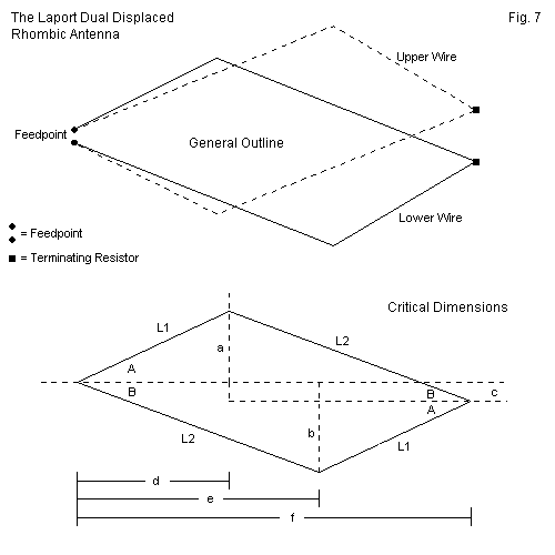
The lower half of the sketch shows the dimensions needed. If we set L1 at 3.5 wavelengths and L2 at 6.0 wavelengths, then angle A becomes 26.1 degrees and angle B is 18.85 degrees. Simple trig relations yield the physical dimensions, including the amount of offset of the far junction from the array centerline (c). To compare the dual rhombic with a single rhombic I scaled my early VHF model down to our test frequency (3.5 MHz) and set it 1 wavelength above average ground. Since the 0.16" wire diameter is much thinner at 3.5 MHz than AWG #12 is at 100 MHz, I set the spacing between wires at 0.08 wavelength and used 900-Ohm terminating resistors in each rhombic in the pair. Even so, the front-to-back ratio is only good, but not optimal. However, the combination of spacing and the terminating resistor values are adjustable in the design to improve these figures without affecting the forward gain or the sidelobe suppression.
The best single rhombic for comparison with the dual version is the model using 5 wavelength legs. It is only slightly longer overall (9.4 wavelengths vs. 8.95 wavelengths for the dual rhombic). The following table presents some of the basic performance data.
A Preliminary Comparison of Equal Length Single and Dual Rhombics
Antenna     Leg Length   Elevation  Max. Gain   Front-Back   Beamwidth   Feedpoint Z
            WL           Angle deg  dBi         Ratio dB     degrees     R +/- jX Ohms
Single      5            13         17.97       44.71        12.8        867 + j23
Dual        3.5/6.0      12         19.82       25.03        12.2        447 + j 9
The feedpoint impedance is the parallel combination of the impedances of the individual offset rhombics in the pair. At VHF and UHF, where the wire is proportionately thicker as a function of a wavelength, dual rhombics would normally use lower values for the terminating resistors and have feedpoint impedances closer to 300 Ohms. The table shows that the dual rhombic has a 2-dB gain advantage over the single rhombic. However, the benefit of the dual design is less the added gain than the sidelobe suppression. Fig. 8 provides elevation and azimuth patterns for the 2 antennas. It also overlays the two azimuth patterns for a more direct comparison of relative sidelobe strength.
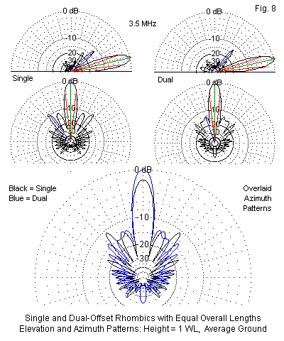
The dual rhombic's strongest sidelobe is about 5-dB weaker than the strongest sidelobe of the single rhombic. We can add 2-dB to that figure when considering the sidelobe strength relative to the strength of the main forward lobe. The sidelobe strength has diminished to a level that equals the sidelobe strength of many (but not all) long-boom Yagi designs with approximately the same forward gain and front-to-back ratio values. For a further discussion of dual rhombics in VHF and UHF service, see Modeling the Dual Rhomboid: Parts 1-3 at my web site.
Conclusion to the Series
The study of long-wire antennas--both terminated and unterminated--is far from complete in these note. There are numerous theoretical directions one can take to intensify one's understanding of the relationship of these antennas to fundamental mathematical concepts governing all antennas. Likewise, both historical practical applications and future possibilities leave much room for exploration, in terms of both available literature and physical experimentation. (I am, for example, unaware of any experiments using dual rhombics in the GHz range, with both rhomboids using copper strips bound to separate sides of a substrate.)
Neverthess, this series of notes has reached its end. Beginning with all-too-often overlooked fundamentals, we explored the basics of lobe formation on both center-fed and end-fed wires ranging from 1 to 11 wavelengths. The galleries of elevation and azimuth patterns should provide a handy reference. At the same time, we looked at the modeling issues and variables involved in portraying long-wire antennas, including changes of ground quality, changes of wire and material, and changes of height. We also saw that as we lengthen a long-wire, the elevation angle of maximum radiation gradually decreased below the traditionally calculated value. We next explored antennas that add a terminating resistor between the far end of the long-wire and ground. These end-fed terminated or traveling-wave antennas formed the simplest fixed beams, although the use of such a resistor reduced the available forward gain relative to unterminated wires of the same length. The terminating resistor largely--but not completely--controls the feedpoint impedance of the antenna, allowing the use of a terminated long-wire beam over 2 or more octaves of frequency change.
The unterminated single long-wire antennas provided us with a critical piece of information in the development of more complex long-wire arrays. The maximum gain for any long-wire antenna does not coincide with the wire end itself, but occurs at an angle that varies with the wire length. V and rhombic arrays depend on this angle to align a major lobe from each individual wire so that the lobes add to increase array gain. Long-wire V antennas are usable in both unterminated and terminated forms. In both cases, the gain is considerably higher than for a single long-wire antenna, and the strongest lobe is in line with the wire. However, the higher gain comes at the expense of beamwidth, as the main lobe becomes very narrow at longer wire lengths. Once more, the terminated V-beam has somewhat less gain than the more bi-directional unterminated V array, but the termination provides considerable bandwidth. The limiting factor for bandwidth is that the leg length changes when measured in wavelengths as the operating frequency changes. As a result, the wire angle no longer is correct for aligning the lobes from the individual wires and the pattern breaks down.
The rhombic is perhaps the largest and most refined of the long-wire antennas, consisting of two Vs, open-end to open-end. The result is 4 wires contributing aligned lobes for higher gain and narrower beamwidth. Although the rhombic suppresses unwanted sidelobes better than the V antenna, significant sidelobes remain. The effort to further suppress the sidelobes has resulted in the development of more complex rhombic designs using multiple rhombic elements offset from each other. Although the unterminated rhombic is usable and has more gain than the terminated version, the gain differential is less than for other types of long-wire antennas. If we optimally design a terminated rhombic--by reference to the correct wire angle relative to the antenna height and leg length--we may obtain at least a 2:1 frequency ratio of high performance at a nearly constant feedpoint impedance.
Although the facts about long-wire antennas are readily available from a variety of sources, these notes have used antenna modeling software as an alternative technique in determining the correct wire angle for maximum antenna performance for any given height and leg length. Starting with the unterminated end-fed long-wire, we can determine the lobe angle and use this information in designing both V and rhombic antennas that use the same wire length for their legs. Although the models used to provide basic comparisons within each antenna type and among types employed a set height (1 wavelength) and lossless wire of a suitable size for the test frequency, modeling software, such as NEC, allows one to vary these elements and rapidly optimize a complete design. Allied to these basic design techniques are methods of placing sources (the feedpoint) and loads (the terminating resistor) to produce accurate calculations without disturbing the basic geometry of the antenna. As the antennas grew more complex, the modeling issues became more significant, although they grew in a stepped fashion with the step-wise increase in the complexity of long-wire antenna geometry.
Long-wire technology dates back to the earliest attempts to control antenna radiation patterns and to obtain gain beyond the levels of single wires. However, the techniques may still have application today and tomorrow. At the same time, modeling design methods can shorten at least some of the calculation time needed to produce a workable long-wire antenna, whatever the type. Our trek through long-wire technology ends here, but the antennas themselves may still have far to go.
Updated 10-01-2006. © L. B. Cebik, W4RNL. The original item appeared in AntenneX for Sep, 2006. Data may be used for personal purposes, but may not be reproduced for publication in print or any other medium without permission of the author.